

An easier (and ‘more statistical’) method
There is an easier method to derive the Phillips model. It invokes a more standard statistical procedure than he himself used.
The proposed model is y = β1x–φ + β2 + ε.
. where x = the annual unemployment rate
. and y = the annual rate of change of wages.
Calculate β1 (the coefficient of x) and β2 (the constant term) from the standard multiple regression matrix formula ß = [XTX]–1XTY. This minimises the sum of the squares of the residual errors (Σε²) for the 53 observations from 1861 to 1913 taken as a vector with 53 rows.
The matrix formula ensures that the regression coefficients will change automatically when Excel Solver is used to re-estimate –φ (the exponent of x). The constraint imposed is to reduce even further the sum of squares of the residuals (Σε²). (Solver is a linear programming technique.)
The econometric model then is
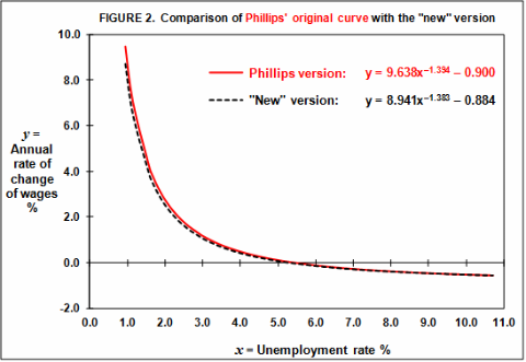
. y = 8.941x–1.383 – 0.884 + ε with R² = 64% (2)
(R² measures how much of the variance in the data is accounted for by the model.)
This new model contains 53 observations with 3 parameters, yielding 50 degrees of freedom. The figure below shows how close this result is to Phillips’ original result.
The experience in modern Ireland
Historically, the labour market in Ireland has tended to be very open. Migration causes an elastic supply of labour and weakens the Phillips Curve effect. The ‘Celtic Tiger’ boom years in Ireland saw a less elastic supply of labour in a move towards full employment. The availability of unemployed labour practically dried up. This strengthened the trade-off between wages and unemployment from 1995 to 2000. The unemployment rate reached an all-time minimum of 3.9% in 2001.
I estimated the annual unemployment rate (x) for the decade that followed from 2000 to 2009, by averaging the corresponding quarterly rates.
To be consistent with Phillips’ logic, I did not take the rate of inflation (y) as the conventional year-on-year change. Rather, I estimated it for each of the ten years by expressing the first central difference of the Consumer Price Index for each year as a percentage of the index for the same year. So I took the rate of change for 2000 as half the difference between the index for 2001 and the index for 1999, expressed as a percentage of the index for 2000, and similarly for the other years.
Then the curve of best fit is y = 60.527x–1.263 – 5.575 + ε with R² = 89% (3)
The figure below shows that the relationship between inflation and unemployment followed the general pattern of a Phillips-like curve from 2000 to 2009. The data points for the eight years from 2000 to 2007 form a cluster corresponding to ‘the good times.’ The first rumblings of the pan-economic depression began to be felt in 2008.
The catastrophic explosion in unemployment to 12% in 2009 resulted from the collapse of the global banking economies in 2008. The implosion of the speculative property market bubble made this worse in Ireland. It had a negative knock-on effect on the construction industry and on the economy in general.

Phillips’ methodology may have been over-complicated, but it is interesting that result2 corresponds closely with the model he proposed1. The main point is that a result quite similar to Phillips’ original model can be derived more simply by combining linear programming with a well-known statistical method. (This simplicity may cause a stir in the econometric world.)
It is 55 years since Phillips published his paper on his curve. Ireland’s experience during the ‘noughties’ shows that, even today, the concept of the Phillips curve can still be relevant. Four years after our economic armageddon, we are still picking up the pieces of our shattered economy.


