
On 21 February 2020, the first person-to-person transmission of SARS-CoV-2 – the virus responsible for Covid-19 – was reported in Italy. After that, the number of people infected with Covid-19 increased rapidly, first in northern regions and then in all Italian territories.
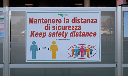
Due to the large increase in cases, the Italian Government introduced a decree on 8 March that placed strong restrictions on movement in the northern regions affected by the epidemic. These restrictions allowed only specific working activities (health- and food-related) and banned any unneccessary outdoors activities. Further decrees on 9 March, 22 March, and on subsequent dates, extended these restrictions to all regions of Italy until 3 May.
Throughout this period, graphs of accumulating cases and deaths have been shown at the daily government press conferences. But these graphs leave us with more questions than answers. As statisticians, we look at them and wonder: “Where are we with Covid-19?”, “What’s going on?” and “Do restrictive measures work?”
To answer these questions, we need to describe the trend of the epidemic. And, in order to understand the evolution of the epidemic, we need models, ones that are, like all models, a compromise between simplicity and accuracy.
The data
Data for Covid-19 in Italy has been available and public since 24 February 2020. Using this data, we set up a team named Robbayes-C19 to model the cumulative numbers of daily deaths (DD) and intensive care unit (ICU) hospitalizations. Our goal is to build a model to read and interpret the (often “unclean”) data that is published daily by the Protezione Civile (Civil Protection services). The aim of the proposed model is to give a general picture of the outbreak, showing the time evolution of daily deaths and intensive care unit hospitalizations, and the effectiveness of the restrictions. Such analyses can provide support for decision making; for instance, the government can decide to modify restrictions when the number of ICU hospitalizations or deaths reaches a certain level on the growth curve.
The daily Protezione Civile data is disaggregated by region. We decided not to consider data on positive daily Covid-19 cases (as a result of a positive swab tested 5-6 days before), since this indicator is likely to be biased towards over-representing cases with severe symptoms and, crucially, by the strength of the testing regime adopted. However, our chosen data sets are by no means perfect. For example, during an epidemic, there is often a delay between the time someone dies and the time their death is reported. Therefore, our DD data must be treated with caution, since it presents large variability and some outliers (see plot on the right-top of Figure 1) due to delayed reporting of deaths.
The model
When working with cumulative data, it is reasonable to consider growth curves. In academic literature, it is known that events whose rate increases initially and decreases later can be well modeled using the so-called log-logistic curve. If, for instance, we look at the cumulative numbers of deaths, we see that at the beginning it increases exponentially and almost seems to explode. After a certain point in time, which represents the inflection point of the curve, the number of deaths continues to increase but more slowly. Studying the shape of this growth curve may help us understand if preventive measures (such as mobility restrictions) can be tightened or relaxed.
Our model assumes that the mean of our variable Y (DD or ICU) has a log-logistic dependence on time (t ) with certain parameters that can be interpreted in terms of the upper limit (i.e. the peak rate of growth), the slope of the curve (i.e. the rate of acceleration/deceleration) and the inflection point (i.e. the point at which growth starts slowing down). The distribution of Y can be assumed to be normal, Poisson or negative binomial. Similar models are also used by other research groups.
Why “robustness”?
Robust statistical methods are not overly affected by outliers or model misspecification. The DD and ICU data must be treated with caution, since it is merged by different local health units and may be affected by different error types in data collection, which may have a serious impact on the estimation of the model – for example, on the slope or the upper limit.1 In particular, DD data present unexpected and unpredictable outliers because of delays in death registration, especially when deaths occur outside hospitals. Moreover, the considered log-logistic model makes strong parametric assumptions about the shape of the curve, the variability and the distribution of Y. To take account of possible deviations from these assumptions, inference on the parameters of the model using this data would benefit from robust procedures.
We follow an approach based on the Tsallis score.2,3 Illustrations of the robust fitted nonlinear models for DD and ICU data are given in Figure 1: the plots to the left show cumulative data from 24 February to 3 May 2020, while the plots to the right show daily counts to see whether we have reached the peak (the mode of the curve). For DD data, the model estimates a total of 33,420 (95% CI: 33,038–33,902) deaths as an upper limit, which will be reached by the end of June, and an inflection point on 6 April. For ICU data, again the model estimates a total of about 188,644 (95% CI: 188,262–189,027) ICU occupancy-days as an upper limit and an inflection point reached on 9 April. Clearly, these fitted models (red lines) cannot be used for predictive purposes, both because of the quality of the data and the restrictions imposed by government, which are subject to change. In fact, the models fit the data well up to 3 May, but it is not possible to predict how the data will change when the restrictions are modified after lockdown ends. However, the plots on the right show that the peak has been reached both for the number of daily deaths (31 March) and daily ICU hospitalizations (2 April), highlighting the effectiveness of the restrictions.
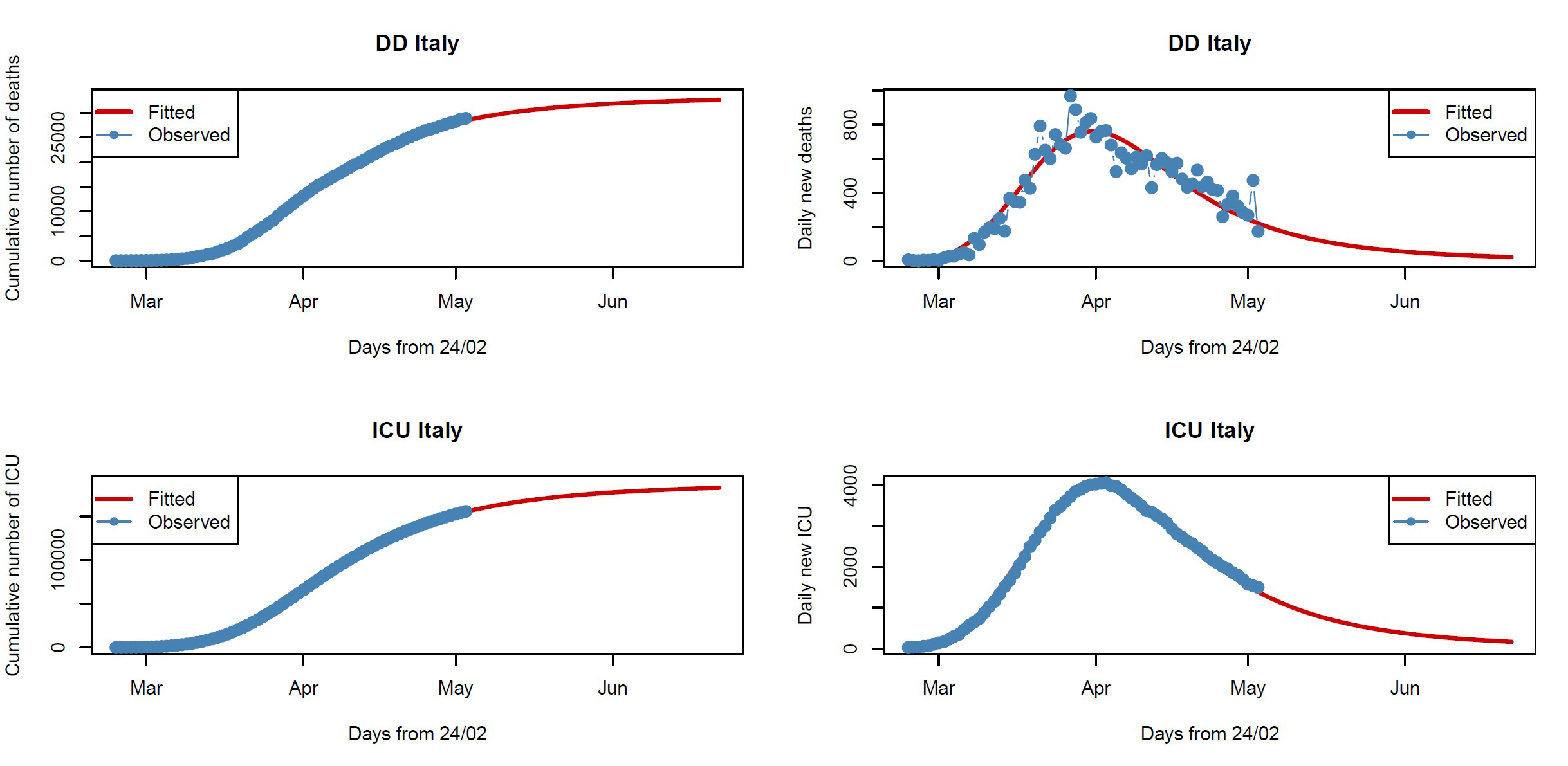
FIGURE 1 Fitted nonlinear models for DD (top row) and ICU (bottom row) data. Blue points are the observed data and red lines the fitted models.
Why use a Bayesian approach?
The Bayesian approach refers to statistical inference where uncertainty in inferences is quantified using posterior probability on the parameters. It allow us to include prior information (objective or subjective) on the parameters of the model, by adjusting the various components of the model based on the information we have at various points in time. Moreover, the plots and analysis of the posterior distributions for the parameters of the model may be quite useful in practice since they may be more informative than a point or interval estimate. For instance, in Figure 2 the marginal posterior distributions allow us to assign probabilities to intervals on the parameters: for DD data, for example, we have a high probability that the upper limit is included in the range 32,000–35,000, while we have a very low probability that it is greater than 35,500.
Mixing robust procedures with the Bayesian approach yields posterior distributions that are resistant with respect to data contamination and model misspecification. Figure 2 gives the violin plots of the robust (SR-post) and classical (called genuine or proper) marginal posterior distributions for the upper limit (left), for the inflection point (center) and for the expected mean (right), both for DD and for ICU data, using an objective prior,4 i.e. a non-informative prior representing prior ignorance. The posterior medians (the white dots) for the upper limits and the inflection points are consistent with the plots in Figure 1. But note that the classical marginal posterior distributions show tails that are too narrow with respect to robust posterior distributions, which, on the contrary, are able to take into account the actual large uncertainty in the available data.
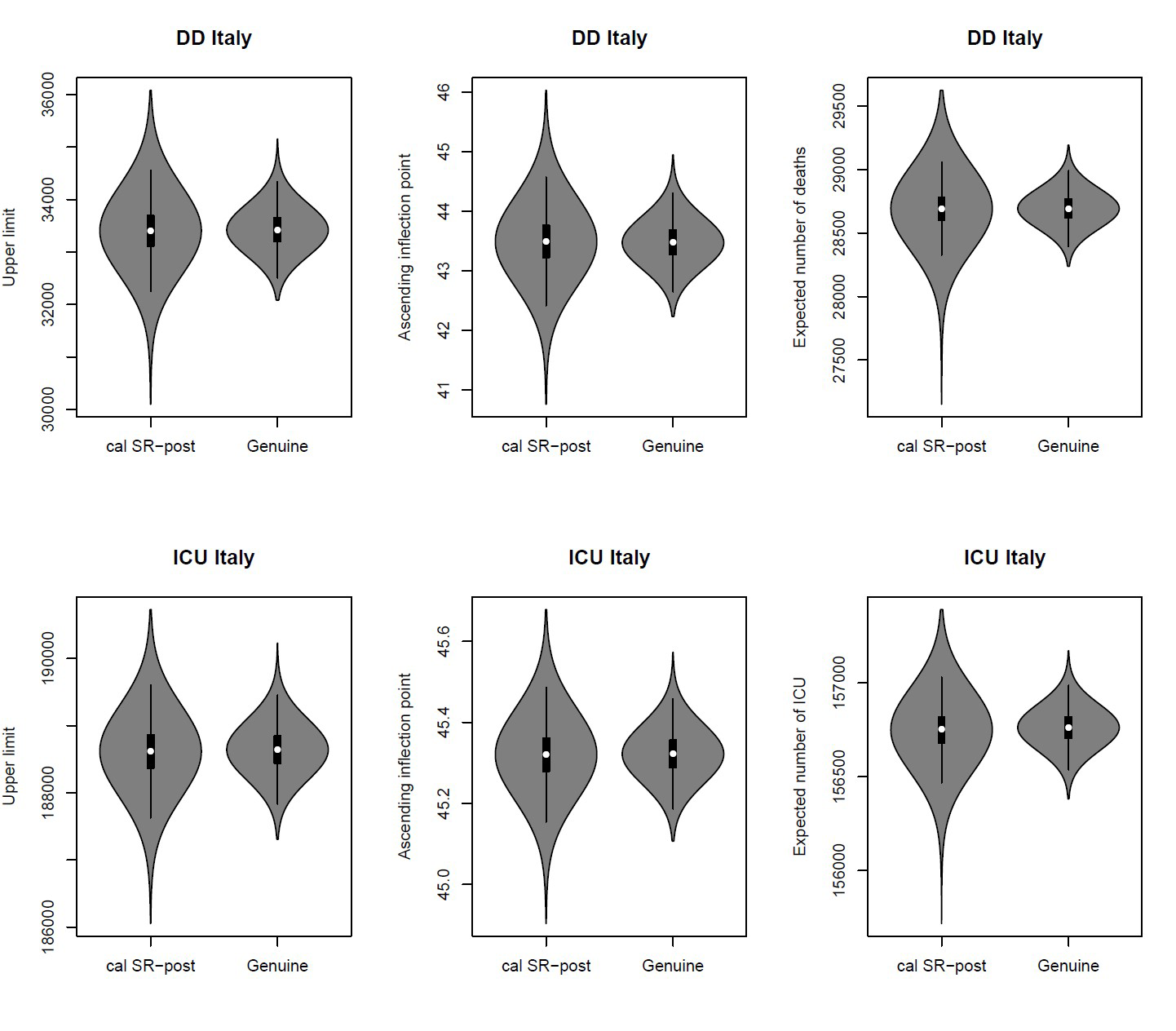
FIGURE 2 Robust posteriors (SR-post) versus the genuine posterior distributions for the upper limit (left), for the inflection point (center) and for the expected mean (right).
Concluding remarks
Our results show how the use of robust and Bayesian methods may be a powerful strategy to overcome errors resulting from real-time data.
From our analyses it emerges that restrictive measures have worked in Italy, since the peak in daily deaths and ICU hospitalizations has been reached. However, the estimation of the model and, as a consequence, the calculation of the expected upper limit and the inflection point are based on the assumptions that the adopted restrictions will not be subject to change. In fact, due to the short incubation period of Covid-19 (on average 5.2 days5), variations in the severity of the restrictive measures can quickly affect the number of infected and, therefore, deaths and hospitalized patients in intensive care units.
The day-by-day monitoring of model fit stability will allow us to evaluate deviations from the actual lockdown situation now that restrictions have started to be lifted.
Note
All the analyses are made with the free software R, version 3.6.1.
Acknowledgements
This research work was partially supported by University of Padova (BIRD197903), by PRIN 2015 (Grant 2015EASZFS_003) and by the Sardinian Region (project STAGE).
About the authors
The authors are all members of Robbayes-C19, a research group spontaneously born in March 2020, composed of researchers from the University of Padua, Udine, Cagliari and Benevento, with robust modeling skills, both in the frequentist and Bayesian frameworks, and experiences of collaborations in medical statistics and epidemiology.
References
- Farcomeni, A. and Ventura, L. (2012) An overview of robust methods in medical research. Statist. Meth. Med. Res., 21, 111-133. ^
- Ghosh, M. and Basu, A. (2013) Robust estimation for independent non-homogeneous observations using density power divergence with applications to linear regression. Electr. J. Statist., 7, 2420–2456. ^
- Dawid, A.P., Musio, M. and Ventura, L. (2016) Minimum scoring rule inference. Scand. J. Statist., 43, 123–138. ^
- Giummolè, F., Mameli, V., Ruli, E. and Ventura, L. (2019) Objective Bayesian inference with proper scoring rules. Test, 28, 728–755. ^
- Wang, H., Wang, Z., Dong, Y., Chang, R., Xu, C., Yu, X., … and Wang, Y. (2020) Phase-adjusted estimation of the number of Coronavirus Disease 2019 cases in Wuhan, China. Cell Discovery, 6, 1-8. ^


