
In December 1971, two years after the successful Apollo 11 moon landing, US President Richard Nixon launched a “war on cancer” with the signing of the National Cancer Act. Since that time, billions of dollars and thousands of careers have been devoted to finding ways to prevent or cure the disease. But the fight is not yet over.
EDITOR’S NOTE This article was a finalist for the 2018 Statistical Excellence Award for Early-Career Writing. Our 2019 competition is now open for entries.
When Nixon’s war began, cancer was the second leading cause of death in the USA. That remains the case today. To intensify this ongoing war, a funding initiative, the “Cancer Moonshot“, was announced during President Barack Obama’s final year in office. The aim was to identify new ways to prevent, diagnose, and treat cancer.
But after all the money and time that has been spent, and with cancer incidence expected to increase in the years to come, a question may come to mind: how many cancers can we actually expect to prevent?
Is cancer simply bad luck?
Mathematician Christian Tomasetti and oncologist Bert Vogelstein addressed this issue in Science in 2015, and fuelled an ongoing, heavy debate.1 They concluded that “only a third of the variation in cancer risk among tissues is attributable to environmental factors or inherited predispositions. The majority is due to bad luck (…)”, a message they repeated in a Science publication in 2017. What are the implications of these findings? Does cancer develop simply due to bad luck or random events? If so, should we withdraw from the war?
Before admitting defeat, we better take a closer look at the arguments presented by Tomasetti and Vogelstein. To do this, we must consider the basics of cancer development.
Human cells normally reproduce by dividing into two daughter cells. In the tissues of a healthy human, there is a delicate balance between old cells dying and new cells arising through cell division. Most cells are not able to divide at all, but there is usually a small population of self-dividing cells, called “stem cells”, that divide in a strictly controlled fashion to maintain the organ function.
Cancer occurs when any type of cell, either a normal body cell or a stem cell, escapes the controlling mechanisms and divides out of control. This uncontrolled growth is caused by changes in the genetic make-up of the cell, and we call these changes “mutations”. So, cancer is fundamentally due to mutations. At each cell division, there is a small chance of a mutation, which may arise without any known external cause. Mutations may also be caused by external factors, such as radiation.
With this in mind, Tomasetti and Vogelstein sought to explain a well-known observation: some types of tissue – for example, those of the breast – give rise to cancer much more frequently than other types of tissue – such as those of the brain. Could this observation be explained by the fact that breast cells divide much more often than cells in the brain? That is, are most cancers simply due to sporadic mutations during the housekeeping of the organ, and not due to external factors?
Tomasetti and Vogelstein showed that the population frequency of cancer in an organ is strongly correlated with the number of stem cell divisions in the organ. The higher the number of stem cell divisions, the higher the probability of a sporadic mutation occurring in the organ.
Consider your subject matter knowledge
You may still be uneasy about the role of chance in cancer development. For example, how can the seemingly random nature of cancer be unified with the strong link between smoking and lung cancer? And if cancer is fundamentally random, why is the risk of skin melanoma, say, much higher in whites than blacks?2
Crucially, Tomasetti and Vogelstein did not claim anything about the importance of different factors for a particular cancer site: they assessed the difference in cancer risk across cancer sites. They did not say that two-thirds of lung cancers are due to chance; they said that two-thirds of the variation in cancer risk between tissues is due to ostensibly random mutations.
To grasp the conceptual distinction, consider the scenario displayed in Figure 1, inspired by a response to Tomasetti and Vogelstein in Nature.3 First, we reproduce results from Tomasetti and Vogelstein: using a subset of their data, we plot the lifetime risk of cancer in a tissue against the number of stem cell divisions in the same tissue (represented as black dots). Now, assume that we introduce an environmental substance in the drinking water (the exposure) such that the risk of cancer in each organ was increased 10 times (red triangles in Figure 1). The correlation coefficient is 0.65 in both scenarios, but in the second scenario everybody has an increased risk of cancer due to the new environmental substance! Hence, the correlation coefficient doesn’t tell us anything about the relative importance of chance for a particular cancer. The correlation coefficient only indicates the difference in cancer risk across organs. This doesn’t give much information about the factors contributing to risk within an organ.
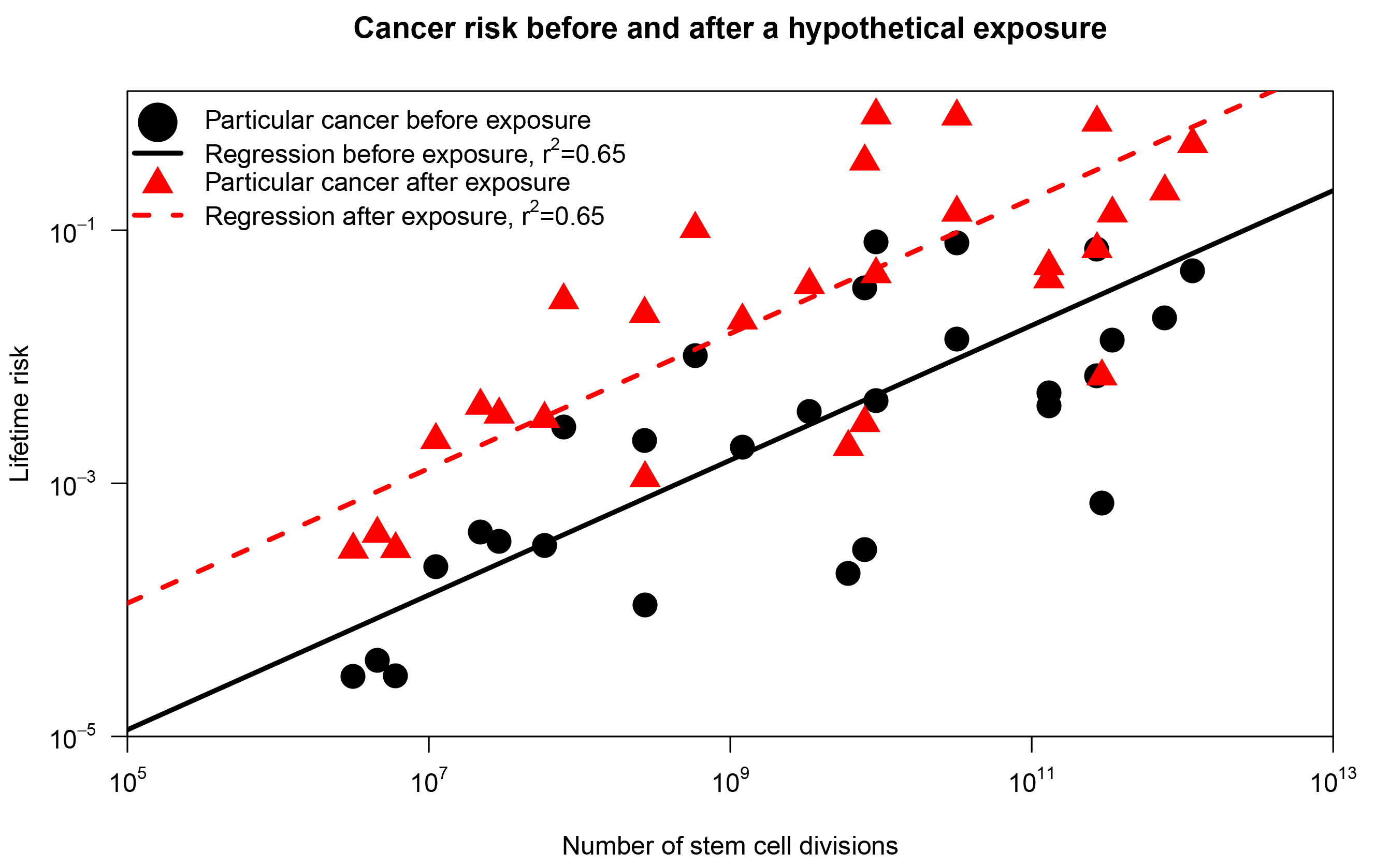
FIGURE 1 The correlation between cancer risk and stem cell divisions. The black dots correspond to the findings of Tomasetti and Vogelstein.1 The red triangles represents the same plot after a hypothetical exposure that increases the lifetime risk of each cancer tenfold.
Take a look at twins
Still, we haven’t yet answered the question of how many (or what proportion of) cancers we can reasonably hope to prevent. We may use available data to approach this question.
If cancer development is purely random, everybody will have approximately the same baseline risk of developing cancer. If there are systematic differences across individuals, these differences must be due to something. This something could, for example, be an unknown environmental exposure, or an unknown genetic factor. To explore such systematic differences, we will consider identical twins.
Identical twins share essentially 100% of their genetic make-up. Since they are born at the same time and usually live under similar conditions, they also share many environmental exposures. We will therefore assume that the probability of acquiring a particular cancer is equal among identical co-twins. This shared probability must be determined by a combination of genes and the shared environment. To make it simple, we will denote all other factors as random. We realise that this is a liberal definition of randomness, because the definition will also cover non-shared environmental exposures. This is also a conservative assumption, because the actual variation in cancer risk is likely to be larger than our estimates.
To illustrate the idea, assume that the identical co-twins Juliet and Emily have a probability of 1.1% of developing pancreas cancer when they are born. That is, this probability, which is unobserved, is shared among the co-twins. If Juliet gets pancreas cancer, despite her low risk, we consider her to be unlucky. If pancreas cancer was purely due to sporadic mutations, without any contribution from genetics or common environment, the risk of pancreas cancer would also be 1.1% in any other twin pair. Then, it would be fair to say that everybody who (randomly) acquired pancreas cancer was really unlucky. However, if the genes and shared environment contribute to cancer, the risk could vary across twin pairs. For example, the co-twins Anthony and Maurits share a genetic predisposition leading to a 60% probability of pancreas cancer. If Anthony gets pancreas cancer, we would hardly attribute the event to random bad luck but to his genetic susceptibility.
Now, let P denote the probability of acquiring pancreas cancer in an individual. For example, Juliet and Emily both had P = 1.1%. We allow P to have different values for different twin pairs. In other words, different twin pairs may have different cancer risk. More formally, we let P follow a continuous probability distribution, describing how the risk is distributed in the population. Indeed, P is a hidden random variable that we usually cannot observe in real-life; most people are not genetically mapped, and the underlying genetic risk of a twin pair (or each individual) isn’t something that we can easily find out.
The population distribution of P, however, must fit with what we observe about pancreas cancer in real-life. First, the distribution must be bounded by 0% and 100%, because everybody must have a well-defined probability of developing the cancer. Second, the mean of the distribution should reflect the observed lifetime risk of pancreas cancer. Indeed, we can use cancer registry data to find that the lifetime risk is 1.1%, and we therefore let the expected value be E[P] = 1.1%. One flexible distribution that accommodates these requirements is the beta distribution.4 This distribution, however, isn’t fully identified by the expected value and the bounding by 0% and 100%. We must also know something about the variance.
To find the variance, we will use a simple trick.5 We will introduce the twin recurrence risk; let’s call it the TRR. This is the probability of getting pancreas cancer given your co-twin was affected by pancreas cancer, divided by the average probabilty of getting pancreas cancer in the population. If acquiring pancreas cancer was completely random, the TRR should be 1; there would be no genetic or environmental factors that puts you at higher risk of pancreas cancer, even if your co-twin was affected. It was just a matter of bad luck. In contrast, a large TRR would indicate that something is influencing the disease risk. We do not know what that something is. Nevertheless, we can estimate the underlying risk distribution if we have information about the TRR. To see this, let E[P2] be the expectation of the probability that both co-twins acquire pancreas cancer, assuming that the co-twins have the same probability of cancer at birth and that everything else that causes cancer is independently distributed across the twins. Then, we use some ideas from Reverend Thomas Bayes to express the TRR:4
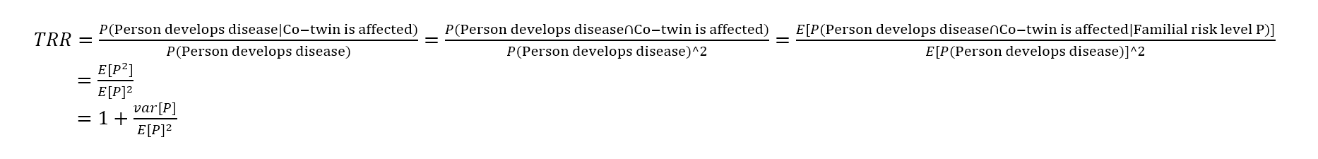
Fortunately, estimates of TRRs are available in the literature. In particular, Scandinavian countries have extensive twin registries and have reported TRRs for various cancers. Here, we will use estimates from a recent, large twin study.6 By inserting the estimated TRR and the lifetime risk into the equation, we solve to find var[P]. Then, we have all we need to see how the risk is distributed in the population, assuming a beta distribution.
Using ideas from Lorenz
We may display the distribution of P in terms of the Lorenz curve. While writing his doctoral thesis on railroad rates, Max Lorenz suggested that this curve may describe the inequality in wealth and income. It is now a standard tool in economics.
The intuition of the curve is straightforward: imagine that we could line up individuals in a country from the poorest to the richest. Then, we plot the cumulative fraction of wealth that is owned by these individuals. If the Lorenz curve is a straight line, all individuals own an equal share of the country’s wealth. The larger the deviation from the straight line, the larger the inequality.
We could do the same for the risk of cancer: we line up people, from those at lowest risk to those at highest risk. Then, the Lorenz curve represents the cumulative proportion of risk, or diagnoses, ‘owned’ by that percentage. For example, the Lorenz curve of pancreas cancer is shown in Figure 2. There is substantial variation in risk, and the 10% at highest risk accounts for 52% of diagnoses. There will, of course, be some uncertainty around the TRR estimate used to produce the curve, and this is also displayed in the figure. But even if the lower bound of the 95% confidence interval is used, the 10% at highest risk would still account for 25% of diagnoses. By looking at the graph in Figure 2, we get the feeling that the risk of pancreatic cancer varies considerably across subjects due to genetic and environmental factors.
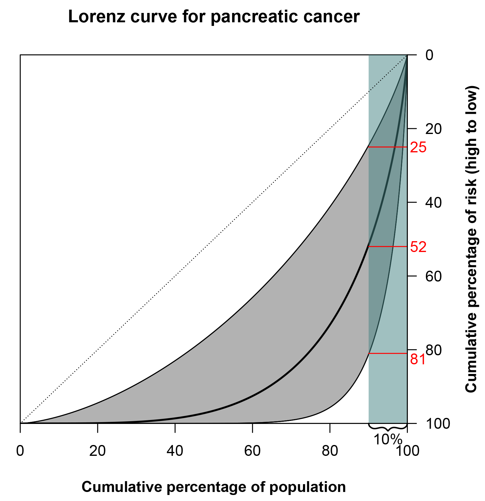
FIGURE 2 Lorenz curve for pancreatic cancer based on a TRR of 3.9.6 The grey shaded area around the curve is bounded by the Lorenz curves constructed from the bounds of the 95% confidence interval of the TRR, 1.4-10.5. The 10% of the population at highest risk (teal-shaded area) accounts for 52% of pancreatic cancers. (The highlighted 25% and 81% correspond to the lower and upper bounds of the Lorenz curve confidence interval, respectively.)
A Lorenz curve may also be summarised in a single number, known as the Gini coefficient, which is perhaps the most popular measure to study inequality in economics. The Gini coefficient is the area between a hypothetical Lorenz curve representing perfect equality and the actual Lorenz curve for a distribution, divided by the area under the perfect equality line. Similar to the Lorenz curve itself, the Gini coeficient is used to assess the inequality in income or wealth in a population, but it is also useful for easy comparison of inequalities – for example, in different countries. Crudely, a Gini coefficient of 0 implies no inequality; a Gini index of 1 denotes complete inequality. The Gini coefficient for pancreas cancer (Figure 3) is 0.71, corresponding to a larger inequality in the risk of pancreas cancer than in the income distribution of the USA (which has a Gini coefficient of 0.41, according to a 2013 estimate from The World Bank).
The case of pancreas cancer isn’t extreme. In Figure 3 the Lorenz curves for cancers of the stomach, ovary, kidney, testis and for melanoma of the skin are presented. All of these cancers have larger inequalities in risk than pancreas cancer.
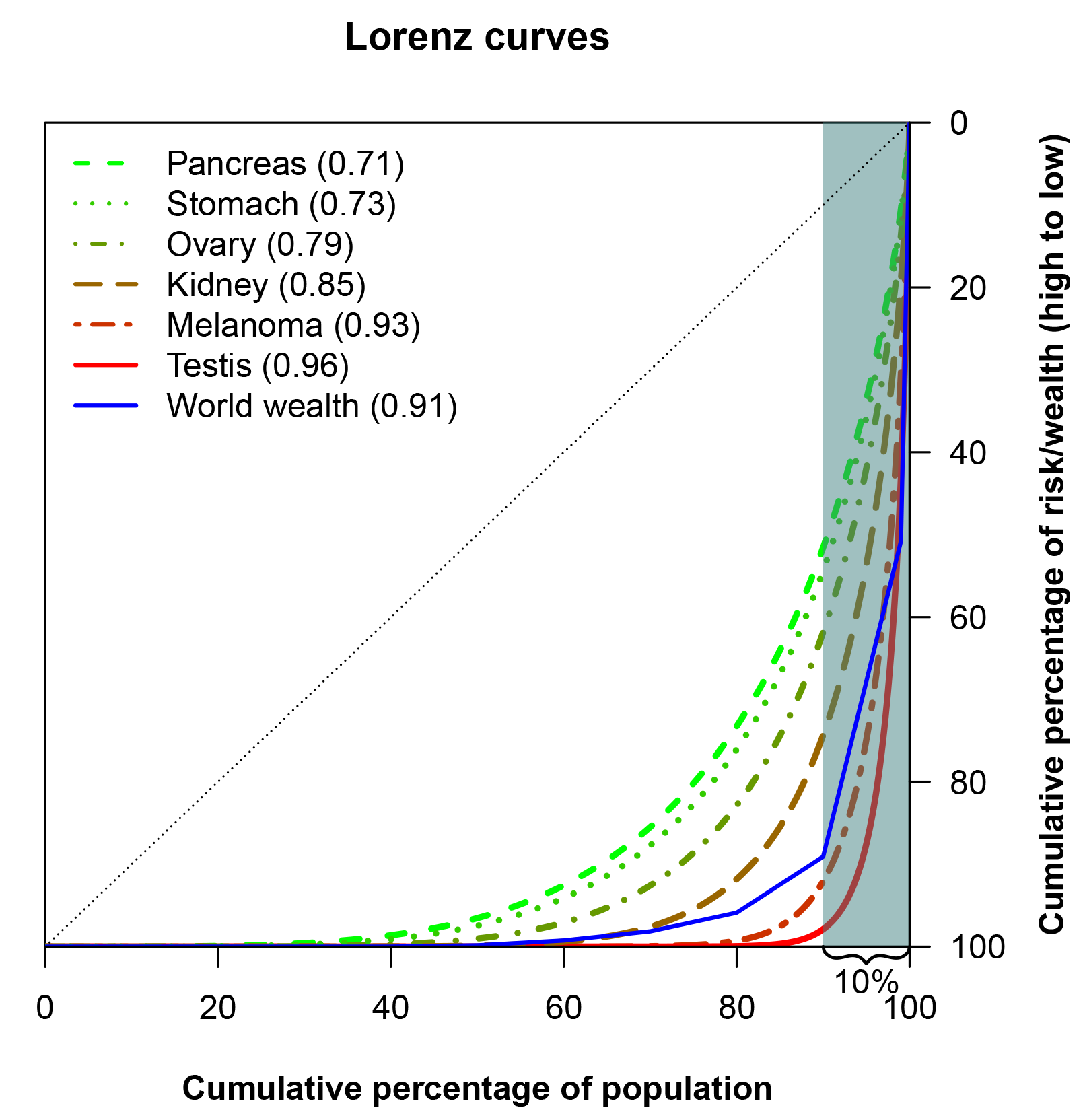
FIGURE 3 Lorenz curves for selected cancers, and for world wealth.6 The Gini coefficients are given in parentheses in the legend.
An Oxfam report, coinciding with the annual meeting of the World Economic Forum in 2017, investigated the distribution of wealth in the world. Across the world there were headlines highlighting that the eight richest men own as much as the poorest 50% of the world’s population. The report also gave the proportion of wealth owned by each decile of the population as well as by the 1% richest, which corresponds to the blue line in Figure 3. It is interesting to see that several cancers have risk distributions that are comparable to, or even more skewed than, the distribution of wealth in the world, when measured with the Lorenz curve.
So, can cancer really be mostly due to simple bad luck? Our considerations suggest not. There seem to be some non-random factors – genetic or environmental – that increase the risk for certain people. These factors may very well vary across tissues, and preventing cancers using a single strategy sounds like an implausible idea. However, the substantial non-random variation in cancer risk between individuals brings us hope: in principle, risk factors for cancers, even if yet unknown, may be targeted by interventions in the future.
Nixon began his “war on cancer” almost half a century ago. Today, with the “Cancer Moonshot” and other continuing efforts, there’s still a chance of victory someday.
About the authors
Mats Julius Stensrud is a postdoctoral researcher the University of Oslo and currently a Fulbright Scholar at Harvard T. H. Chan School of Public Health. His main research interest is causal inference in medicine. He also holds a medical degree, and he used to work as a resident doctor in internal medicine.
Morten Valberg is a postdoctoral researcher at the Oslo Centre for Biostatistics and Epidemiology, University of Oslo and Oslo University Hospital. He completed his PhD in biostatistics at the University of Oslo in 2014. One of his main research interests lies in the modelling of unobserved heterogeneity in survival analysis.
References
- Tomasetti C, Vogelstein B. Variation in cancer risk among tissues can be explained by the number of stem cell divisions. Science. 2015;347(6217):78–81. ^^
- Cormier, Janice N., et al. Ethnic differences among patients with cutaneous melanoma. Archives of internal medicine. 166.17 (2006): 1907-1914. ^
- Wu S, Powers S, Zhu W, Hannun YA. Substantial contribution of extrinsic risk factors to cancer development. Nature. 2016;529(7584):43–47. ^
- Valberg M, Stensrud MJ, Aalen OO. The surprising implications of familial association in disease risk. BMC public health. 2018;18(1):135. ^^
- Stensrud MJ, Valberg M. Inequality in genetic cancer risk suggests bad genes rather than bad luck. Nature Communications. 2017;8(1):1165. ^
- Mucci LA, Hjelmborg JB, Harris JR, Czene K, Havelick DJ, Scheike T, et al. Familial risk and heritability of cancer among twins in Nordic countries. JAMA. 2016;315(1):68–76. ^^^


