

On 31 December 2019, the World Health Organization (WHO) was alerted to an unusual cluster of pneumonia patients in the city of Wuhan, China. Clinical signs and symptoms included fever and breathing difficulties; chest radiographs revealed invasive lesions of both lungs. Some of the early patients were vendors in Wuhan’s Huanan seafood wholesale market, where live wild animals were also being sold illegally, and where the new disease is suspected to have originated.
Now known as Covid-19, the disease has spread rapidly around the world, first to other countries in Asia and then on to the Pacific, Europe, Africa, and the Americas. By the time the Covid-19 event was officially characterised a “pandemic”, on 11 March 2020, the disease had been documented in 114 countries, territories and areas, and the associated case count had exceeded 118,000.
As the first waves of SARS-CoV-2, the viral agent of Covid-19, began to reach the United Kingdom, the British government published a four-stage national plan to tackle its spread. The plan began with attempted containment of infections, before moving onto plans to delay spread, to conduct research and, finally, to mitigate the health and economic consequences of the infection.
Effective implementation of a strategy which involves the containment and/or the delay of spread of a disease such as Covid-19 assumes an ability to model the rate at which an infection spreads, both through time and space. There are well-established methods for assessing the rate of temporal growth by, for example, looking at the trajectory of case doubling times or estimating the propensity for a single case to generate new cases in a population – the so-called basic reproduction number, R0. In terms of cases, R0 is interpreted as the average number of secondary infections produced when one infected individual is introduced into a wholly susceptible population. The crucial point here is that measures such as doubling times and R0 are essentially aspatial – they tell us very little about the rate the disease or virus is spreading in different parts of a country or region. The issue becomes especially acute when plans for, say, the relaxation of lockdown conditions include an explicitly geographical dimension – with restrictions perhaps being lifted in certain areas before others.
In such scenarios, we need a spatial or geographical equivalent of R0. But defining one is not straightforward. Time is a unidirectional metric from past to present to future. Space, however, is multidirectional in its behaviour. A virus can jump in any direction from a source to other areas and back again; there is no natural order as there is with time.
Disease geographers at Cambridge and Bristol have, however, made some progress by defining a suitable spatial R0 which is denoted as R0A.1 The principles underpinning the approach are illustrated in a box (below). But to explain simply and by direct analogy with R0, the method takes all the geographical units in a study area (A) at any time point in an epidemic and groups them into one of three states: infected are those areas in which cases are present, recovered are those in which the epidemic wave has passed through, and susceptible are those which the epidemic wave has yet to reach. This information is then used to define velocity parameters which measure how rapidly the so-called “leading edge” (VLE) of an epidemic reaches susceptible areas and how soon the wave passes through (represented by the “trailing edge” or “following edge” (VFE) of the wave). The equation for R0A (see box) shows that the parameter compares the arriving velocity of the disease wave with the departing velocity, with the difference between the two indicating whether the infection wave speeded up or slowed down when passing through.
Testing the model: pandemic influenza in France
As we are in the midst of the Covid-19 pandemic at the time of writing, we have limited data with which to demonstrate how R0A applies to this particular disease. However, we can illustrate the model with reference to the historical record of influenza pandemics and epidemics in France.
Like Covid-19, influenza is a viral respiratory disease for which the primary mechanism of transmission is via exposure to respiratory droplets. But the similarities between the two diseases should not be overstated; they differ in terms of their clinical course, symptoms and prognosis. An understanding of the distinct challenges associated with the spatial modelling of Covid-19 await the availability of more data.
In France, data on influenza deaths – by time (weeks, months, years) and by area (towns, départements, regions) – have been either collected or estimated by the Ministère de l’Intérieur and related bodies since 1887, making them one of the longest continuous spatially disaggregated influenza time series in the world (Figure 2).2
The influenza pandemics to which the population of France (and elsewhere) was exposed in the late nineteenth and twentieth centuries are summarised in Table 1. As in most countries, the 1918–19 pandemic stood alone in France in terms of the mortality caused. While the long-term trend in influenza mortality depicted in Figure 2 was steadily downwards, it was the case that pandemic years generally experienced heightened mortality as compared with adjacent years.
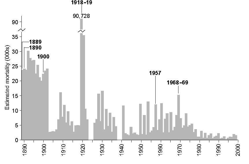
FIGURE 2 Influenza mortality in France, 1887–1999. Time series of annual deaths from influenza reported in French records. The millennium is taken as a convenient end date for the present analysis.
TABLE 1 Influenza pandemic events, 1887–1999.
| Year(s) | Virus subtype | Colloquial name | Notes |
| 1889–90 | A/H2N? | First deaths were reported in France in November 1889; the peak month was January 1890. | |
| 1900 | A/H3N? | It has been queried whether this was a true global pandemic event. Excess mortality was reported in North America and in England and Wales, but not globally. | |
| 1918–19 | A/H1N1 | “Spanish” influnza | This pandemic produced a level of mortality so far unequalled in recorded history. The event occurred in three main waves: Wave I (April–July 1918); Wave II (August–December 1918); Wave III (March 1919). |
| 1957–58 | A/H2N2 | “Asian” influenza | This pandemic occurred in two main waves: Wave I (February–December 1957); Wave II (November 1957–March 1958). |
| 1968–70 | A/H3N2 | “Hong Kong” influenza | This pandemic occurred in two main waves: Wave I (1968–69); Wave II (1969–70). Wave I primarily affected North America and to a lesser extent Europe. In Wave II, the situation was reversed. |
So how rapidly did these influenza pandemics, and intervening epidemics, spread throughout the geographical areas of France? Using monthly data at the spatial scale of département (95 in total), Figure 3A plots annual estimates of the spatial basic reproduction number R0A and the two edge parameters, VLE and VFE . The trend lines show that the long-term direction in R0A was slowly downwards during the twentieth century. That is, the rate of geographical spread of influenza epidemics gradually diminished, probably reflecting less intense epidemics arising from (i) improved standards of living and healthcare, and (ii) no major changes (“shifts”) in the genetic structure of influenza A viruses after 1969 that would enable them to by-pass existing immunity in the population. This century-long declining trend in R0A is reflected in a similar decline in the leading edge velocity parameter (VLE ), and a rising trend in the following edge parameter (VFE ), implying that epidemics arrived later and ended sooner in each influenza season; in essence, influenza seasons became of shorter duration as the twentieth century progressed.
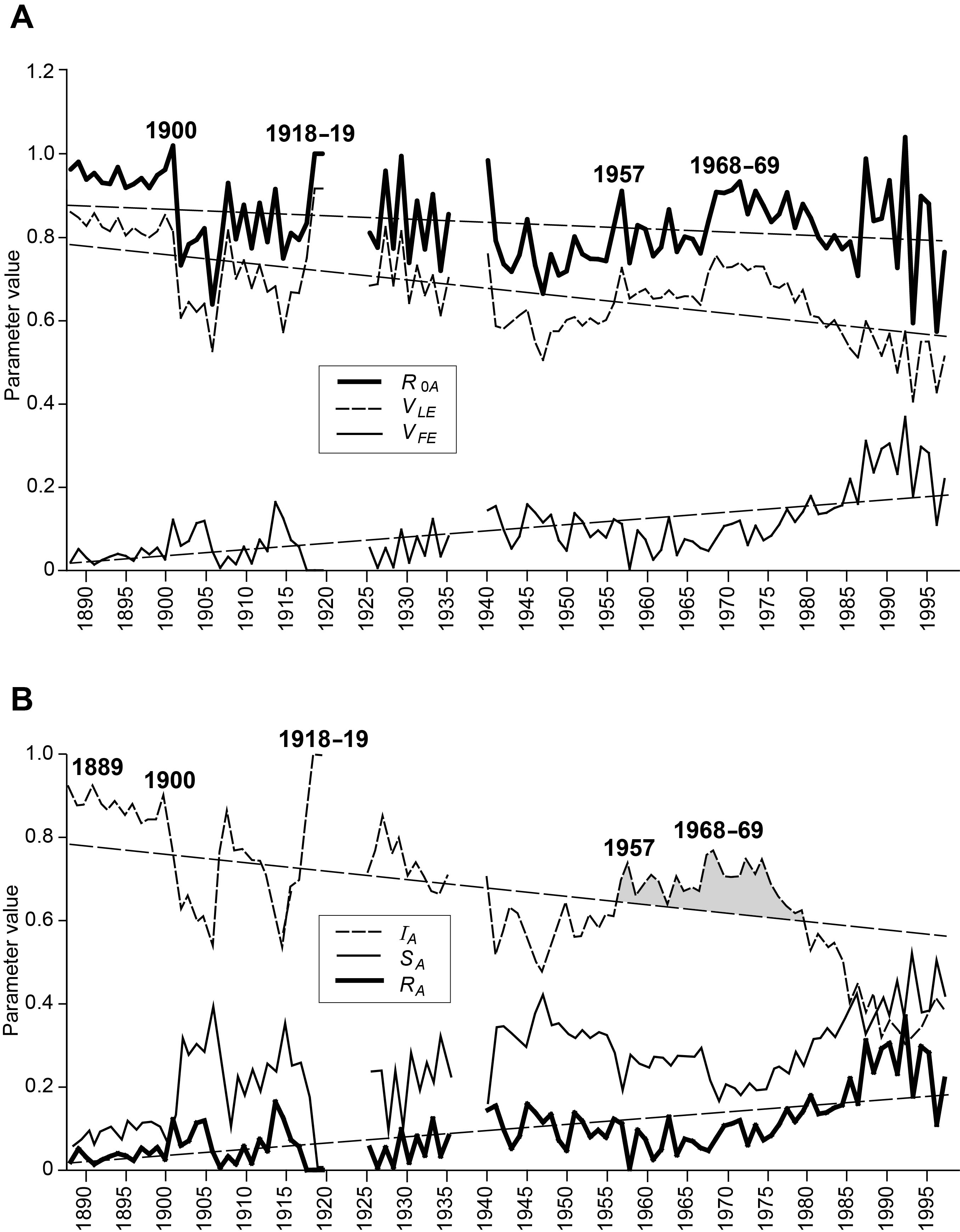
FIGURE 3 Swash model parameters for influenza in France, 1887–1999. (A) Time series plots of calculated values for the spatial basic reproductive number, R0A, and for the edge velocity parameters, VLE and VFE . (B) Time series of the infected (IA), susceptible (SA) and recovered (RA) integrals. Linear regression trend lines are also shown. See box for an explanation of the measures.
Within these long-term trends, however, the pandemic seasons of 1900, 1918–19, 1957 and 1968–69 showed locally raised values of R0A, thereby signalling the heightened rate of geographical spread of the novel influenza viruses with which these events were associated. Interestingly, this is not evident for the 1889–90 pandemic, while the rise to a higher level in 1968 persisted for four seasons and is consistent with Viboud and colleagues’ characterisation of a “smouldering pandemic”.3 From the late 1980s, R0A oscillated wildly, suggestive of locally intense epidemics in each influenza season involving only a few départements rather than the entire country.
Table 2 highlights the difference between pandemic and non-pandemic seasons in France. The seasons have been classified into three groups: (i) pandemic-affected (11 seasons); (ii) high-intensity inter-pandemic (54), with death rates greater than the lowest pandemic season; and (iii) low-intensity inter-pandemic (38), with death rates lower than the lowest pandemic season. The leading edge velocity parameter (VLE ) in Table 2 confirms that the rate of spatial propagation declined systematically as between the pandemic (0.80), high-intensity inter-pandemic (0.70) and low intensity inter-pandemic (0.59) seasons. The higher velocity of pandemic seasons was maintained even when compared with inter-pandemic influenza seasons of similar intensity levels. Moreover, pandemic seasons appeared to be of greater spatial intensity (larger R0A) and were slower to clear (lower VFE ).
TABLE 2 Characteristics of 103 influenza waves: France 1887–88 to 1998–99.
| Leading edge (LE) velocity | Following edge (FE) velocity | |||||
| Type of influenza wave | Death rate1 | t̄LE (months) | VLE | t̄FE (months) | VFE | R0A (mean) |
| Pandemics (n = 11) | 27.29 | 2.39 | 0.80 | 11.45 | 0.05 | 0.93 |
| Interpandemic | ||||||
| High intensity (n = 54) | 14.91 | 3.59 | 0.70 | 11.20 | 0.07 | 0.84 |
| Low intensity (n = 38) | 3.14 | 4.93 | 0.59 | 10.12 | 0.16 | 0.80 |
1Seasonal average, expressed per 100,000 population.
The time series plots in Figure 3B depict the proportion of French départements in each of the susceptible (SA), infected (IA) and recovered (RA) states at the end of each influenza season. The plots for SA and RA show rising trends over the decades, and this is consistent with the generally declining trend for IA . Effectively, as the decades wore on, fewer départements were infected by influenza in a given season and, if they were infected, they transitioned more rapidly to a state of recovery. Again, the pandemic years bucked the trend with raised values of IA , indicating a tendency for greater proportions of départements to be infected by pandemic waves and for the disease to persist in these areas for longer.
The main other variations in the long-term fall in IA occurred following the arrival of the “Asian” influenza pandemic in 1957, when the IA remained above the trend line (shaded) until its precipitous fall in the 1980s. The extended period of higher values for IA from the late 1950s to the late 1970s may be attributable to the combined action of three effects: (i) the long interval since the last major shift in virus subtype (40 years since 1918); (ii) the shift from the A/H2N2 to the A/H3N2 virus with the arrival of the “Hong Kong” influenza pandemic in 1968; and (iii) the re-emergence in 1976 of the “Russian” influenza (A/H1N1) virus which has been co-circulating with the Hong Kong (A/H3N2) virus ever since. Together these effects meant that a greater proportion of the French population was likely to be susceptible to one or other of the mix of circulating subtypes than if just a single subtype had been present over the period. After a generation, with no new major virus subtypes emerging, herd immunity appears to have caught up from the mid-1980s, leading to a general collapse of nationwide epidemics.
Conclusion
Trialling the spatial R0A and related parameters (see box) on French influenza data suggests that it can separate pandemic, epidemic and other seasons, so that it can be used to inform decisions about the public health preparations which need to be made to restrict pandemic spread.
Obviously, the model will need wider testing and refinement using different geographical settings and diseases to establish its utility and robustness. But at this early stage it appears to give new spatial perspectives on infection transmission to complement existing (aspatial) approaches.
As far as Covid-19 is concerned, until a safe and effective vaccine is developed and licensed, control of spread in all countries is being exercised by a mixture of self-isolation, quarantine and lockdown so that transmission chains from infected populations to susceptible populations are severed – methods developed in Italy during the plague centuries from c.1300–1800.
The first major assessment of the efficacy of these methods for Covid-19 has appeared in The Lancet, focusing on China’s cities and provinces outside the source province of Hubei.4 The authors used an instantaneous reproduction number, Rt , in a SIR (susceptible, infectious, recovered) model and found that the disease transmission rate fell sharply after 23 January, when restrictions on personal interactions were introduced, but that relaxation of the restrictions allowed Rt to rise again.
Spatial analogues of the reproduction number could add an important dimension to the ongoing monitoring and assessment of SARS-CoV-2 transmission in both its expansion and retreat phases, and could inform geographically-based decisions over the relaxation of lockdown conditions.
BOX The spatial basic reproduction number, R0A
Statistical details of R0A and related parameters are given elsewhere.2 Figure 1 illustrates the underlying principles. We begin, in Figure 1A, with a hypothetical 12 area map in which areas are identified as a1, a2, . . , and 10 time periods indexed as t1, t2, . . . This is converted into a space-time data matrix in which 122 recorded cases of a disease are distributed to simulate an array typical of an epidemic wave. For any one of the rows in the data matrix, two cells can be identified which mark the “start cell” and the “end cell” of a recorded outbreak. Figures 1B and C analyse these start and end cells. In Figure 1B, the matrix is re-arranged so as to position the start cells in an ascending temporal order. This line of cells (dark shading) defines the position of the leading edge (LE) that marks the start of the epidemic wave in the different areas. To the left and above this line lies a zone of cells (light shading) which have yet to be infected and thus may be regarded as areas to which the epidemic has yet to spread. Similarly, the matrix can be organized as in Figure 1C, so as to arrange the end cells in ascending temporal order. This line of cells (dark shading) defines the position of the trailing edge or following edge (FE), marking the completion of the epidemic wave in the different areas. To the right and below this line lies a zone of cells which have ceased to be infected and which thus may be regarded as areas which have recovered from infection.
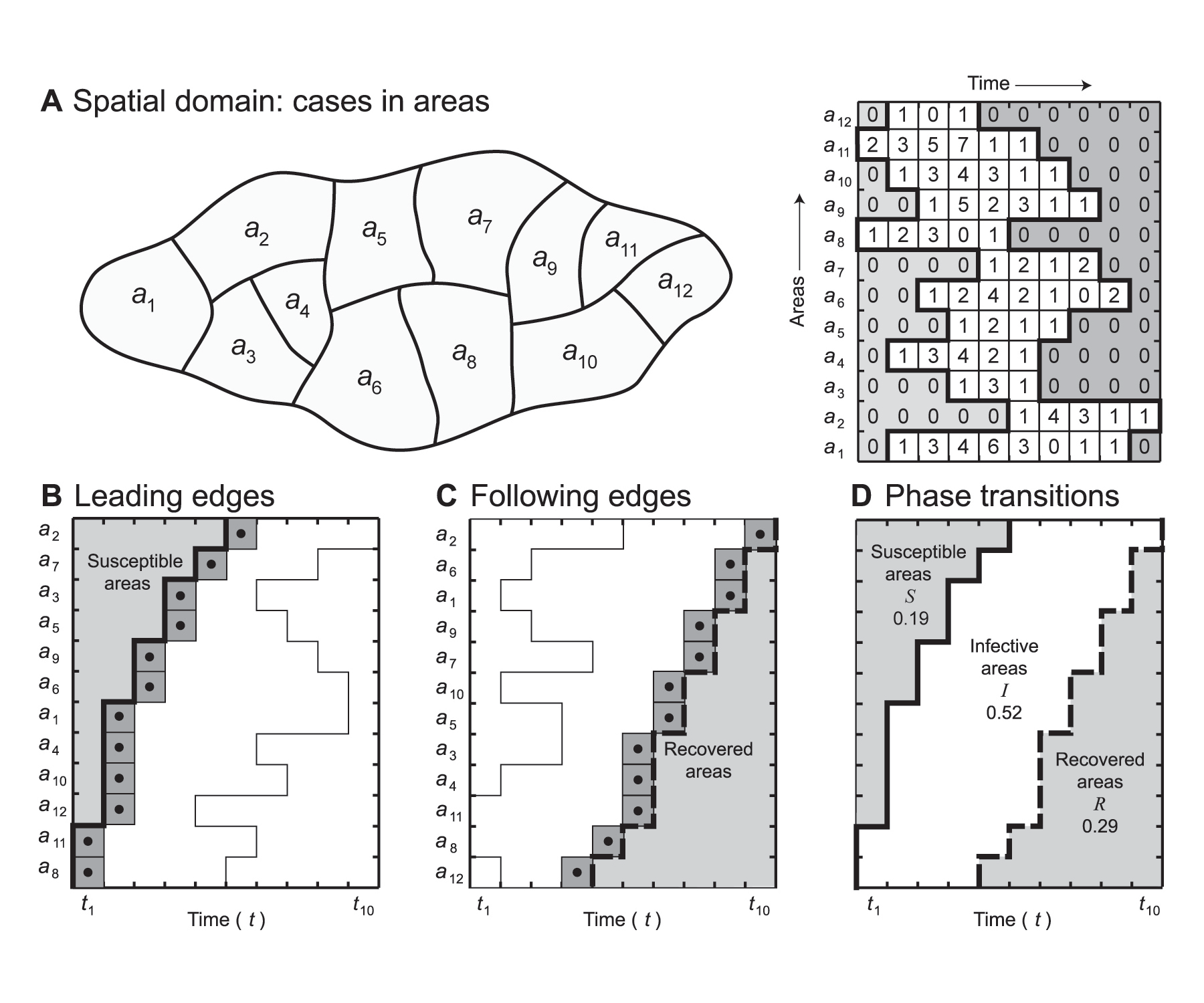
FIGURE 1 Spatial basic reproduction number, R0A: hypothetical example. (A) Base map and space-time disease matrix. (B) Matrix arranged to order leading edges (LE). (C) Matrix arranged to order following edges (FE). (D) Leading and following edges plotted as a phase transition diagram.
Both the edges, LE and FE, can be combined as in Figure 1D to identify cells (areas) which are in susceptible (S), infected (I) and recovered (R) states. This is an exact analogy with infected, susceptible and recovered individuals when defining R0 in a human population rather than in a population of geographical areas. The resulting graph may be regarded as a phase transition or SIR diagram. It has two roles: first, it defines the boundaries of the two phase shifts from susceptible to infective status (S ⇒ I) and from infective to recovered status (I ⇒ R); second, it integrates the three phases, S, I and R, as areas within the graph. The phase diagram has characteristic configurations depending upon the velocity, duration and ultimate spatial extent of an epidemic wave as it passes through a region.
For each edge in Figure 1D, we can define a time-weighted arithmetic mean, t̄LE and t̄FE , which gives the average time of arrival (LE) and departure (FE) of the infection wave across the set of areas. These time-weighted means can be converted to dimensionless velocity ratios VLE and VFE with values in the range [0, 1].
For the time-space map in Figure 1D, the integral SA defines the proportion of areas at risk of infection and is given by
SA = (t̄LE – 1) / T,
while the integral IA defines the proportion of areas that are infected and is given by
IA = (t̄FE / T ) – SA .
Finally, the integral RA defines the proportion of areas in the recovered state and is given by
RA = 1 – (SA + IA ).
All three integrals are dimensionless numbers with values in the range [0, 1] such that SA + IA + RA = 1.
The spatial basic reproduction number R0A is derived from the integrals SA and RA in the manner
R0A = (1 – SA ) / (1 – RA ).
Effectively, R0A provides a measure of the propensity of an infected geographical unit to spawn other infected units in later time periods. Values of R0A calibrate the spatial velocity of disease spread, with higher values denoting more rapid spatial propagation.
References
- Cliff, A. D. and Haggett, P. (2006) A swash-backwash model of the single epidemic wave. Journal of Geographical Systems, 8(3), 227–252. ^
- Cliff, A. D., Smallman-Raynor, M. R., Haggett, P., Stroup, D. F. and Thacker, S. B. (2009) Infectious Diseases. Emergence and Re-emergence: A Geographical Analysis. Oxford: Oxford University Press, 549–597. ^ ^
- Viboud, C., Grais, R. F., Lafont, B. A., Miller, M. A. and Simonsen, L. (2005) Multinational impact of the 1968 Hong Kong influenza pandemic: evidence for a smoldering pandemic. Journal of Infectious Diseases, 192(2), 233–248. ^
- Leung, K., Wu, J. T., Liu, D. and Leung, G. M. (2020) First-wave COVID-19 transmissibility and severity in China outside Hubei after control measures, and second-wave scenario planning: a modelling impact assessment. The Lancet Online DOI: https://doi.org/10.1016/S0140-6736(20)30746-7. ^
About the authors
Matthew Smallman-Raynor is professor of geography at the University of Nottingham.
Andrew Cliff is emeritus professor of geography at the University of Cambridge.


