When an Instagram influencer asked a rhetorical question about probability, statistician and crochet fan Sarah Lotspeich could not resist answering it
I often find inspiration through social media – cute cat photos, yummy recipes, and inspiring travel locales. I have also crocheted for most of my life, fancying myself not only a statistician but a stati-stitchin, and I often find free patterns on social media, too. Most recently, my worlds collided in a new and exciting way: A crochet influencer on Instagram (@krochet.by.kris) asked a statistics question! She had recently undertaken a new project, called “Mystery Daisy Cardigan.” She was crocheting classic “daisy granny squares” (Figure 1), but here’s the catch! Her 4 yarn colours – for the centre, petals, background, and border – were chosen randomly. Then, she would stitch the daisies together into a cardigan.
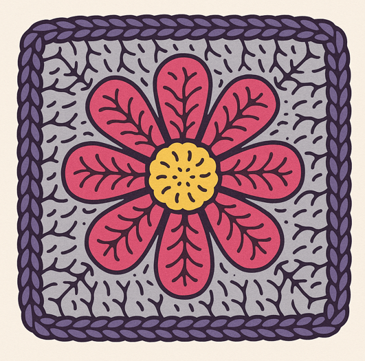
Figure 1: Illustration of a crochet “daisy granny square” in four colours (center, petals, background, and border). Image generated by ChatGPT (DALL·E), OpenAI, 2025.
Riveted, I watched weeks of videos in a matter of minutes. Over time, the inevitable conflict arose: Some colours clashed (looking at you, dark orange). Worse yet, why, cruel fate, did those colours seem to be the ones that kept getting chosen? “What’s the probability of that?” cried @krochet.by.kris into the internet void over a pile of orange-riddled daisy squares. As a lover of both crochet and probability, I had to bring her peace by answering this haunting question.
Setting up the stitcher’s sample space
Since the yarn colours were randomly chosen, the Mystery Daisy Cardigan presents a nice opportunity to illustrate the sample point method in probability.1 In statistics, experiments don’t always take place in a lab – we define them as the generating process leading to the data we see. In this case, the data are the crocheted squares (described by their 4 colours), and the crux of how they get generated lies in @krochet.by.kris randomly choosing colours.
Each iteration of the experiment results is a finished daisy square, which we call our sample point. Before things get mathier, we need a nice symbolic way to denote the different squares. There are a few considerations for these symbols: (i) they need to reflect all 4 colours chosen and the flower parts for which they were chosen, and (ii) they need to be short, sweet, and to the point.
I chose to start by letting each yarn colour be denoted by a single letter and use lower- versus upper-case letters to distinguish between light and dark shades, respectively (Figure 2). Then, a daisy square’s 4 colours can be represented by a 4-letter sequence, where the letters’ order is dictated by the parts: centre, petals, background, and border. For example, the square in Figure 1 would be encoded as “YPrR” for its dark yellow centre, dark pink petals, light purple background, and dark purple border.
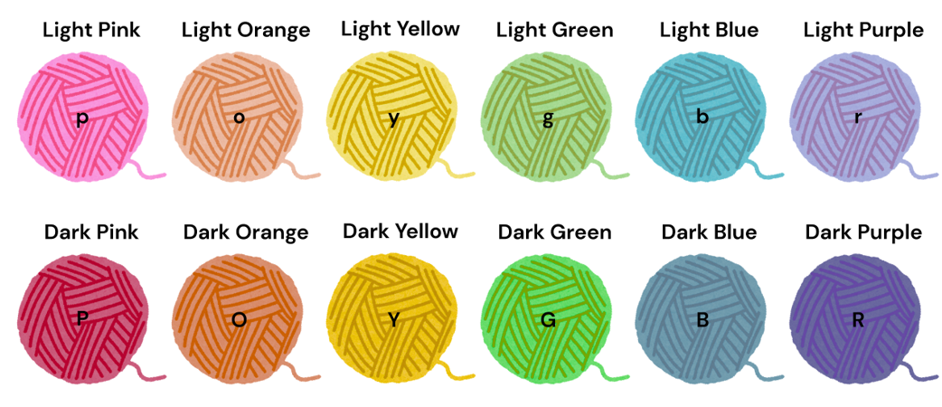
Figure 2: Define a letter to represent each yarn colour in our sample point (daisy granny square), with light and dark colours distinguished by lower- and upper-case letters, respectively.
From stitch counting to the mathematical study of counting
Before calculating the probability of particular events – like an unfortunate preponderance of dark orange – the last thing we need to do is count the total number of possible 4-colour squares. In other words, we need to define the size of Mystery Daisy Cardigan’s sample space, the set of all our experiment’s potential outcomes. So, how hard can counting all those squares really be?
Well… it depends on several factors, including (i) how many yarn colours we’re choosing from (@krochet.by.kris used 12) and (ii) how many colours we’re using for one square (4). You could certainly start your counting by trying to list all the possibilities in an organised fashion, like in Table 1.
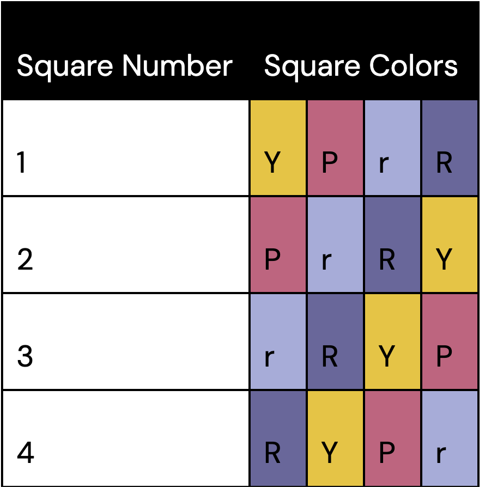
Table 1: Organised way to list possible four-colour yarn combinations for daisy squares.
But it can become very tedious to list sample points when there are lots of possibilities, and there’s always a chance of missing some. Fortunately, we have nice ways of counting the total number of sample points in the sample space without having to list them all, thanks to combinatorics: the mathematical theory of counting.
To get down to the numbers, we need to count the number of ways that we can pick 4 yarn colours from 12 options, but we still have a couple of questions to answer.
1. Can a yarn colour be chosen more than once for the same daisy square?
No, we want maximum colour in the cardigan, so once a colour has been chosen for part of the daisy (like the middle) it is removed from consideration for other parts (like the petals, background, or border). In other words, yarn colours are chosen without replacement for each part of the daisy square.2
2. Should two daisy squares be counted as the “same” if they share the same colours assigned to different parts?
No, to celebrate the uniqueness of the daisy squares, we want to distinguish them by not only the colours included but also their placement. That is, when drawing our 4 yarn colours, their order matters since the first colour determines the centre, the second the petals, and so on.2
Thus, the size of the sample space is equal to the number of ways to pick 4 yarn colours from 12 options, uniquely assigning each colour to at most one flower part. Based on this information, we have the following numbers of choices for each part:
- Centre: 12 colour choices,
- Petals: 11 remaining colour choices,
- Background: 10 remaining colour choices, and
- Border: 9 remaining colour choices.
Altogether, every time colours are chosen, 12 x 11 x 10 x 9 = 11,880 possible daisy squares could be created. We get this number from the fundamental theorem of counting, which says that if there are 12 ways to do the first task, 11 to do the second, 10 to do the third, and 9 to do the fourth, then there are 12 x 11 x 10 x 9 ways of doing all 4 together! Aren’t you glad we didn’t try to write them all out? Now, let’s dig into the main event (the probabilities).
The foundation row: Probabilities about a single square
One important feature of this experiment is the random selection of the yarn colours for each square. Relying on randomness means that each of those 11,880 possible daisy squares has equal probability, and – in fact – this probability is super tiny!
Pr(Any Particular Square) = 1 / Total Number of Squares = 1 / 11,880 (< 0.01%)
While this news might be disappointing if you’re rooting for any of your favorite colour combinations, it’s super useful in calculating other probabilities. So, let’s get to @krochet.by.kris’s original question about how likely we are to see the same colour. While we discuss these probabilities in reference to that pesky dark orange, the values are the same for any particular colour!
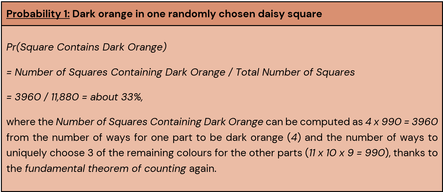 So, there’s a pretty high (33%) probability of getting dark orange in a particular daisy square! Fortunately, it’s still more likely that we will not get it, though.
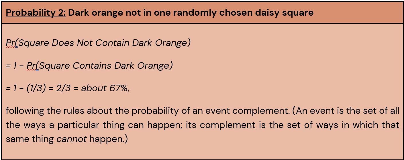 Together, we can use Probabilities 1 and 2 to compute the odds of getting dark orange in a randomly chosen daisy square. Odds are distinct from probabilities – even though the two words are often used interchangeably in popular culture – and can be uniquely useful, particularly for interpretation.
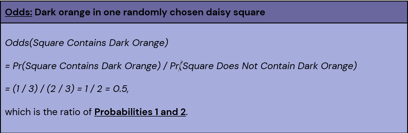 With odds of 0.5 (or “1-to-2”), we are twice as likely to not draw dark orange for a randomly chosen square as we are to draw it. Now, let’s scale things up to multiple squares.
Probabilities of matching colours
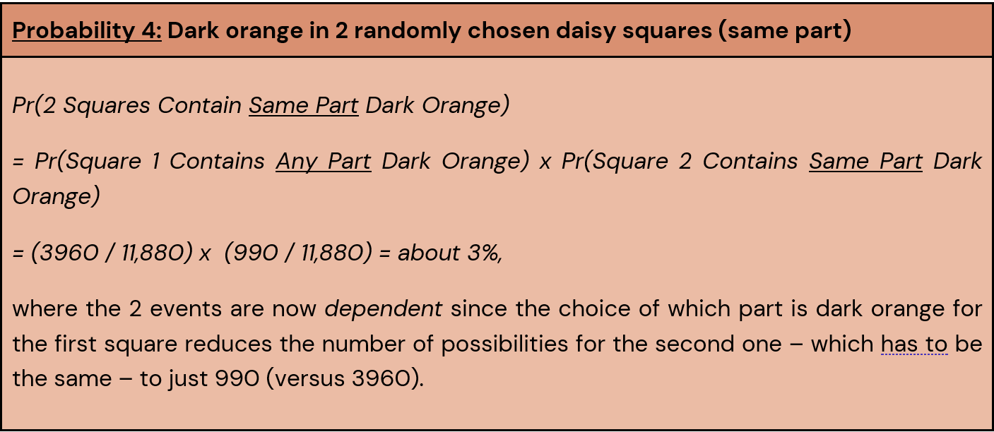
OK, so maybe our chances of getting dark orange on 1 square are higher than we’d like. But – to @krochet.by.kris’s original question – what’s the probability that we get 2 of them?
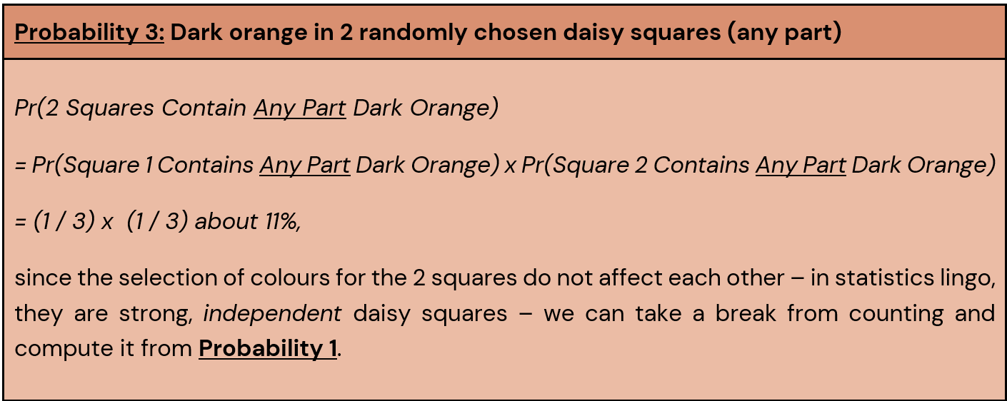 Yikes, at 11% it’s probably more probable than we’d like to randomly draw dark orange for not just 1, but 2 daisy squares! If it’s any comfort, this probability shrinks a lot if we focus on getting dark orange in the same part of 2 daisy squares.
 That’s a bit of a relief! Maybe the dark orange isn’t terrible for all flower parts? Having just a 3% probability of getting 2 daisy squares with it in the exact same place gives me hope.
Speaking of hope… it might be natural to think that if we just made a daisy square with dark orange, we might be “safer” (i.e., less likely) to get it again on the next one! There’s a name for this phenomenon, both in statistics and psychology. When an individual (erroneously) believes that a random event is more or less likely to happen based on what did or did not happen previously, they have fallen to the gambler’s fallacy.3 This is another place where independence between the colour draws comes into play.
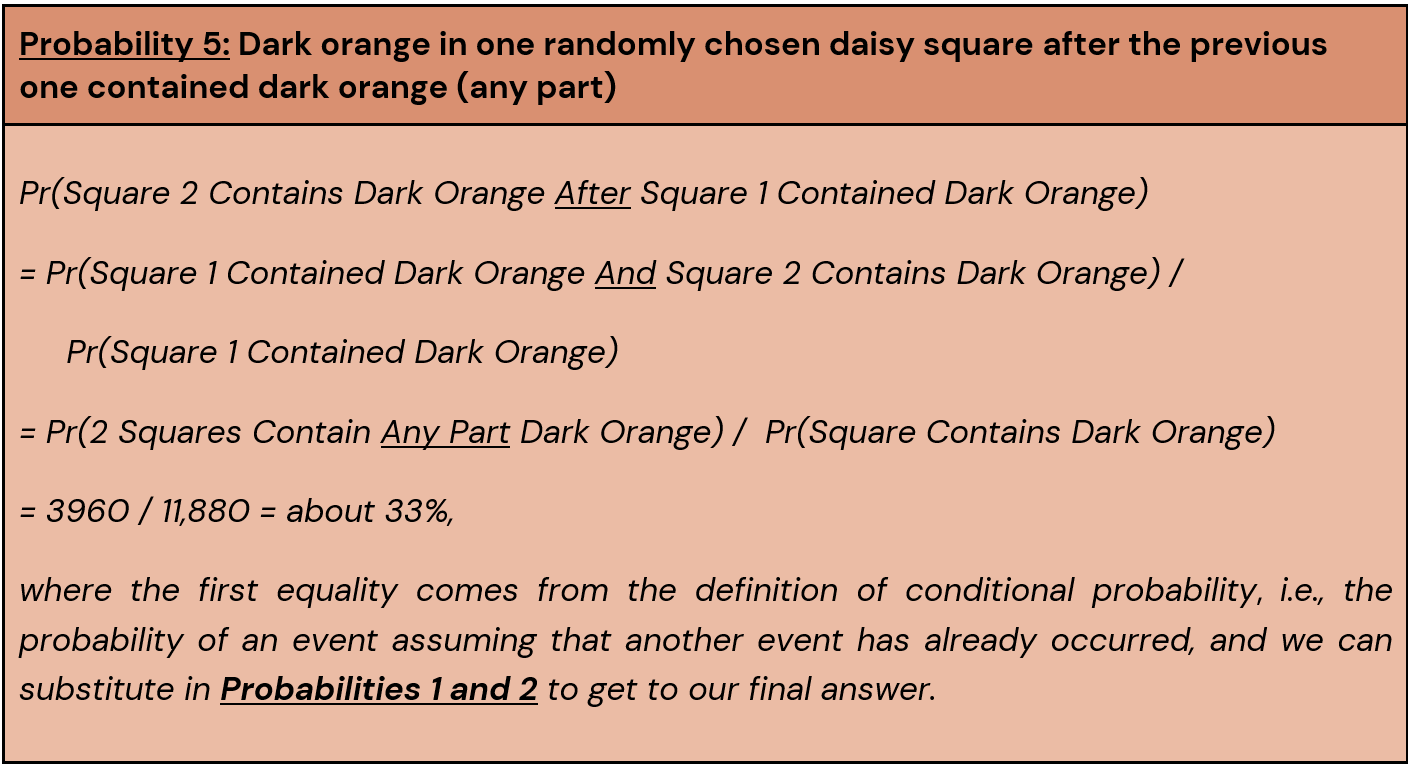 No matter what squares have come before, the probability that the next one will contain that dreaded colour will always be the same: 33%. The squares’ independence implies that Pr(Square 2 Contains Dark Orange After Square 1 Contained Dark Orange) is just equal to Pr(Square 2 Contains Dark Orange). But what if we once again were interested in the dark orange being in the same part?
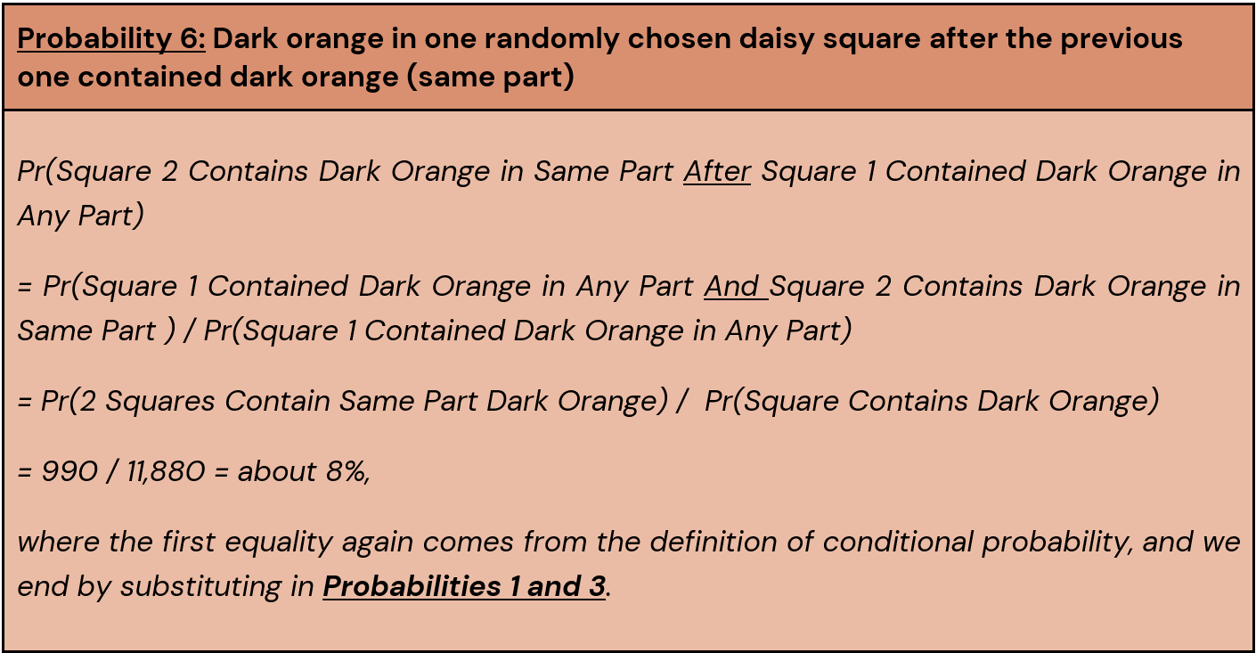 So, if we’re worried about getting dark orange in the same part on the next daisy square, it is true that we have a smaller probability relative to our standard probability of getting dark orange (8% versus 33%).
Wrapping up with the finished cardigan
We can use Probabilities 1 – 6 to extend our thinking to the finished Mystery Daisy Cardigan. Suppose that @krochet.by.kris made 24 squares before assembling. Across the sweater, what is the probability of seeing dark orange a particular number of times? How many times would we have expected it to appear? To answer these questions, it’s helpful to upgrade the Mystery Daisy Cardigan experiment to the Mystery Daisy Cardigan Binomial Experiment.
Each of the 24 squares is considered an independent trial (an iteration of the experiment) that can be summarised by a binary outcome (something with two possibilities, like “yes” or “no” this square contains dark orange). Moreover, each of the 24 squares has the same 33% probability of being a “yes” and containing dark orange, so the trials are identical.
Now, I promise the vocabulary lesson is worth it because binomial experiments have their own well-established formulas that we can use to find the probability of having a particular number – let’s call it y – of dark orange squares in the finished cardigan, where y can be anything from 0 (no dark orange) to 24 (all dark orange).
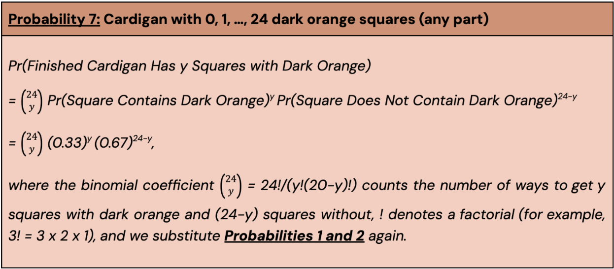 For authenticity, I revisited @krochet.by.kris’s latest post and counted 8 daisy squares with dark orange in the final cardigan. Using Probability 7, this much dark orange had a 17% chance of occurring, which might feel small. However, we actually would have expected to see dark orange appear in 24 x 0.33 = 7.92 daisy squares, following the expected value formula for the binomial experiment. That is, if we repeated this experiment lots of times, making lots of sets of 24 squares and assembling them into cardigans, we expect the average number of dark orange squares across them to be approximately 8.
So, I am sorry to report that what we saw – unfortunately – seems pretty likely. Maybe the safest thing would be to make sure you love all yarn colours equally before hopping on this rollercoaster.
References
- Wackerly, D. D., Mendenhall, W., & Scheaffer, R. L. (2008). Mathematical statistics with applications. Belmont, CA: Thomson Brooks/Cole.
- Casella, G., & Berger, R. L. (2002). Statistical inference. Belmont, CA: Duxbury.
- Kenton, W. (2023) Gambler’s Fallacy: Overview and Examples. Investopedia. www.investopedia.com/terms/g/gamblersfallacy.asp
Sarah Lotspeich is assistant professor at Wake Forest University, Winston-Salem, NC, U.S.A. This article was a finalist for the 2025 Statistical Excellence Award for Early Career Writing. The 2026 writing award closes for submissions on 31 May 2026.
You might also like: Autism, Bayesian probability, and why we do what we do


