In 2007, Netflix launched the second iteration of its annual competition where, for the grand prize of one million dollars, participants attempted to outperform the company’s movie recommendation system based on an anonymized dataset consisting of users’ viewing history and ratings. While the dataset was designed to protect users’ privacy, within a few weeks researchers at the University of Texas at Austin were able to re-identify a large number of users by combining the dataset with public ratings on websites like IMDB. Netflix was forced to cancel the competition in 2009 following a series of lawsuits alleging that the company had violated federal privacy laws.
The Netflix Prize fiasco was a high-profile case demonstrating the risk of re-identification for anonymized data through other publicly available sources. And while we’ve all probably watched a few things on Netflix that we’d prefer to keep to ourselves, our medical records or responses to a census or health survey are far more sensitive and constitute a much graver privacy risk if they could be publicly tied back to us. As the culture of research shifts to facilitate the sharing and publishing of rich, individual-level datasets containing personal information, and if simply anonymizing a dataset is insufficient to preserve an individual’s privacy, should we be creating entirely fake data instead?
Microdata
Every year countless private and governmental organizations collect detailed individual level information through various methods like surveys, censuses or clinical trials called “microdata”. Confidentiality agreements between the collectors and participants often do not allow for the sharing of this data with external parties. There also exist prescriptive regulations like the Health Insurance Portability and Accountability Act (HIPPA) in the US and the General Data Protection Regulation (GDPR) in the EU which explicitly prohibit the sharing of sensitive personal information.
However, the ability to release versions of this data to the public would have substantial benefits to society. It would facilitate the democratization of science and push for open access by providing researchers across the world with high quality data which they could integrate into their own research while tackling problems of high societal significance, and codify the belief that publicly funded research should in fact be freely available to the public. It would also alleviate some of the concerns with the current reproducibility crisis by allowing independent parties to verify the results of existing research before its results shape policy or the health of millions of individuals.
We cannot, of course, neglect the substantial dangers and privacy concerns that arise from sharing such sensitive data, and inherent in this dilemma is the perpetual challenge we have always faced of balancing the rights of the individual with the good of the collective. So what can be done to facilitate the sharing of high quality microdata while also preserving the privacy of an individual?
Data anonymisation
The first and most obvious step would be to simply strip a dataset of any information that is personally identifiable. This would include unique identifiers like ID or Social Security Numbers, and variables which may become personally identifiable when combined with other variables. For example, the combination of first name, last name, age and zip code could very well be unique and re-identified when combined with external data sources like civil registry files. In some cases, even combinations of age, ethnicity and zip code could also be unique. Stripping the dataset of all demographic information would render it useless for analysis, so a common technique is to reduce the granularity of the data by collapsing variables like age and income into categories and replacing specific geographic information like zip codes with larger geographic units.
But as we saw with the Netflix Prize, even a dataset stripped of all this information is not foolproof when combined with other sources. So not only does anonymizing data not eliminate the inherent re-identification risks, it also forces us to either completely discard valuable data or reduce its detail and lose important information. Could we instead create entirely synthetic data which both preserves the core statistical relationships in a dataset while mitigating or even eliminating any possible privacy risks?
Synthetic data and the Cooperative Election Study
The use of statistics and machine learning to create synthetic data which appears to be real has garnered significant media attention recently in the context of deep fakes and the spread of disinformation. These techniques are broadly categorized as “generative methods”. While some are rooted in more traditional statistics and others in newer advancements in the field of deep learning, they all share a common goal: learning an underlying joint distribution for a set of variables from real data and then sampling from that derived distribution to create fake data. To illustrate what may seem like a complex procedure, we turn to the Cooperative Election Study (CES).
The CES is an annual, publicly available and anonymized survey of over 50,000 people in the US electorate consisting of hundreds of questions designed to measure public opinion and attitudes towards social issues. Suppose we are interested in studying the relationship between supporting Donald Trump in the 2020 presidential election for a subset of around 7.5k verified voters who took part in the survey in 5 key swing states, with respect to variables like race, gender, age, party identification and who an individual voted for in the 2016 election. The section below describes the simplest approach and general intuition behind how to build a synthetic dataset.
The first step in our iterative process is to simply choose one of the variables and obtain its observed “marginal” distribution. To keep things simple, we start with the states and the observed marginal distributions would simply be the proportion of respondents in the survey coming from each of the 7 states. We then choose a second variable and obtain its “conditional” distribution after observing the first variable, or in our case we could consider the proportion of respondents of each race within each state. We would then consider a third variable like gender and obtain its conditional distribution after knowing that respondent’s state and ethnicity. By repeating this process of selecting variables, deriving the distribution of the next variable, and iterating through all the variables, we end up with a series of conditional distributions which capture the key statistical dependencies and joint distribution of the data.
To create a synthetic observation from our data, we iteratively sample from these distributions to build out a new row. In our case, the first step would be to randomly sample a state using the marginal distribution of states in the raw data. So, if approximately 15% of respondents came from Arizona and 20% came from Florida, we would randomly select one of these states with 15% and 20% chance respectively. Now that we’ve randomly selected a state, we would then randomly select race using the conditional distribution of race given that sampled state. If, for example, we selected Arizona and approximately 40% of the respondents from Arizona were White and 20% were Hispanic, we would randomly select one of these two ethnicities with 40% and 20% chance respectively.
By continuing this iterative process known as “simple synthesis”, we eventually sample the last variable in our data using all the previously sampled variables to obtain a fully synthetic observation. By repeating this process, we can generate as many synthetic observations as desired, all of which are, by construction, random and therefore no longer contain any information that could be re-identified back to any specific individual.
While this type of simple synthesis that uses proportions is, as the name suggests, rather simple, more sophisticated techniques rooted in both parametric and non-parametric statistics can be used to model each distribution like classification and regression trees, random forests, Bayesian networks or any other machine learning algorithm.
So, if creating these synthetic datasets is rather easy, the question that remains is, how well do they maintain the core statistical relationships and how reliable will inferences made off of them be?
How fake is real enough?
Assessing the quality of synthetic datasets boils down to two main questions: how well does the synthetic data resemble the original data, and how reliable will the inferences made about the population be?
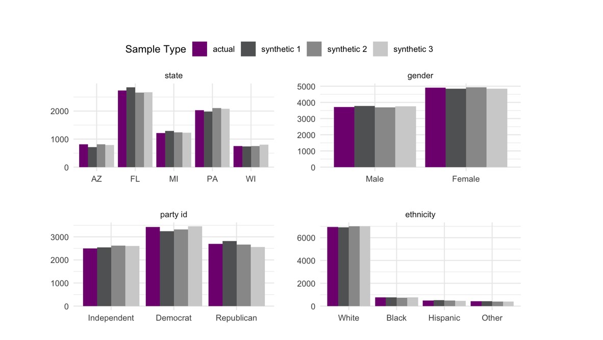
To answer the first question, the simplest approach would be to look at the overall marginal distributions of the key variables in the synthetic dataset and compare them to their marginal distribution in the original dataset. The figure below shows these distributions for state, gender, ethnicity and party identification with three synthetic datasets generated from the CES.

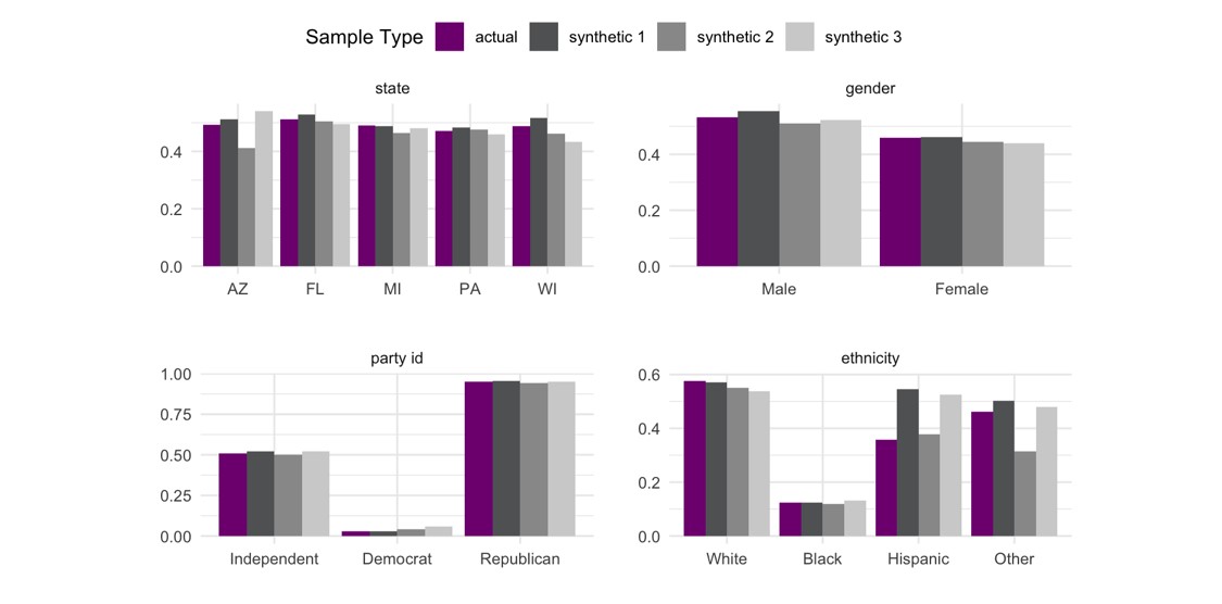
Overall, the distributions in the three synthetic datasets look relatively reasonable when compared to the original data, but ultimately we’re much more interested in evaluating whether the relationships between these variables are maintained rather than just their marginal distributions. As we’re predominantly interested in whether an individual supported Donald Trump, a simple check would be to compare the proportion of support for Trump with respect to these variables in the original and synthetic datasets.

While the three synthetic datasets show some variability in their topline proportion of support for Trump, the key trends in the original data are still present and the extremely low support from voters who identify as Democrats and high support from Republicans is particularly encouraging. We notice that some categories within ethnicity like Hispanic and Other, and the state of Arizona show a much higher variability than other variables which is largely driven by the relatively small sample sizes for these groups.
The process of sampling from these distributions to generate synthetic datasets is random, just like the process of sampling from a population to create a sample, meaning it’s possible to end up with a bad synthetic dataset just like it’s possible to end up with a bad survey. These errors are exaggerated when the sample sizes or members of a target population are small.
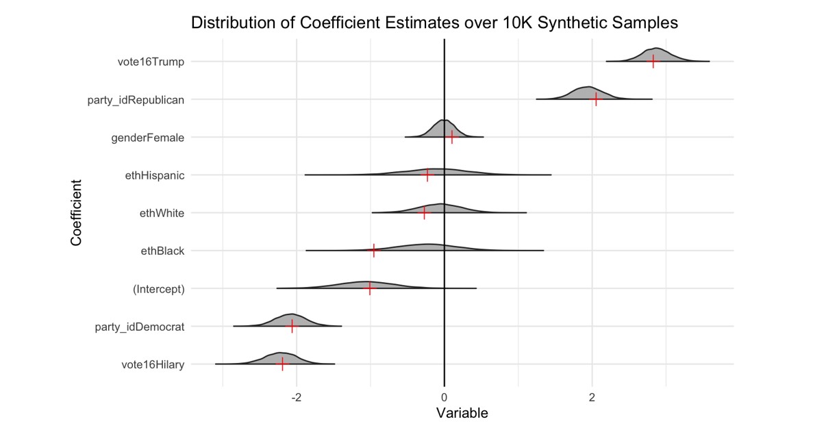
The previous plots only tell us part of the picture, they don’t actually tell us whether all the key dependencies in the dataset are maintained. To evaluate the entire structure of the data, a more rigorous yet simple approach is to fit a logistic regression to the raw data with a binary indicator for support for Trump as the response variable and race, gender, age, party identification and who an individual voted for in the 2016 election as the predictors. We can then compare the coefficients obtained from fitting the same model to a synthetic dataset, and this comparison does, in fact, capture the whole structure of the data and tells us how well we’d be able to study our question of interest with a synthetic dataset. For this analysis, we generate 10,000 synthetic copies of our voters and compare the distribution of the coefficients from these datasets to coefficients from the raw data which are shown in red.

We see that, on average, the models built from the synthetic datasets generally produce similar results to the original data and the estimates are generally consistent with conventional wisdom on how we would expect voters to behave. Some of the variables which had low sample sizes have much wider tails in their coefficient estimates, and this is likely related to how synthesizing data for subsets of the sample with few responses can lead to higher variance.
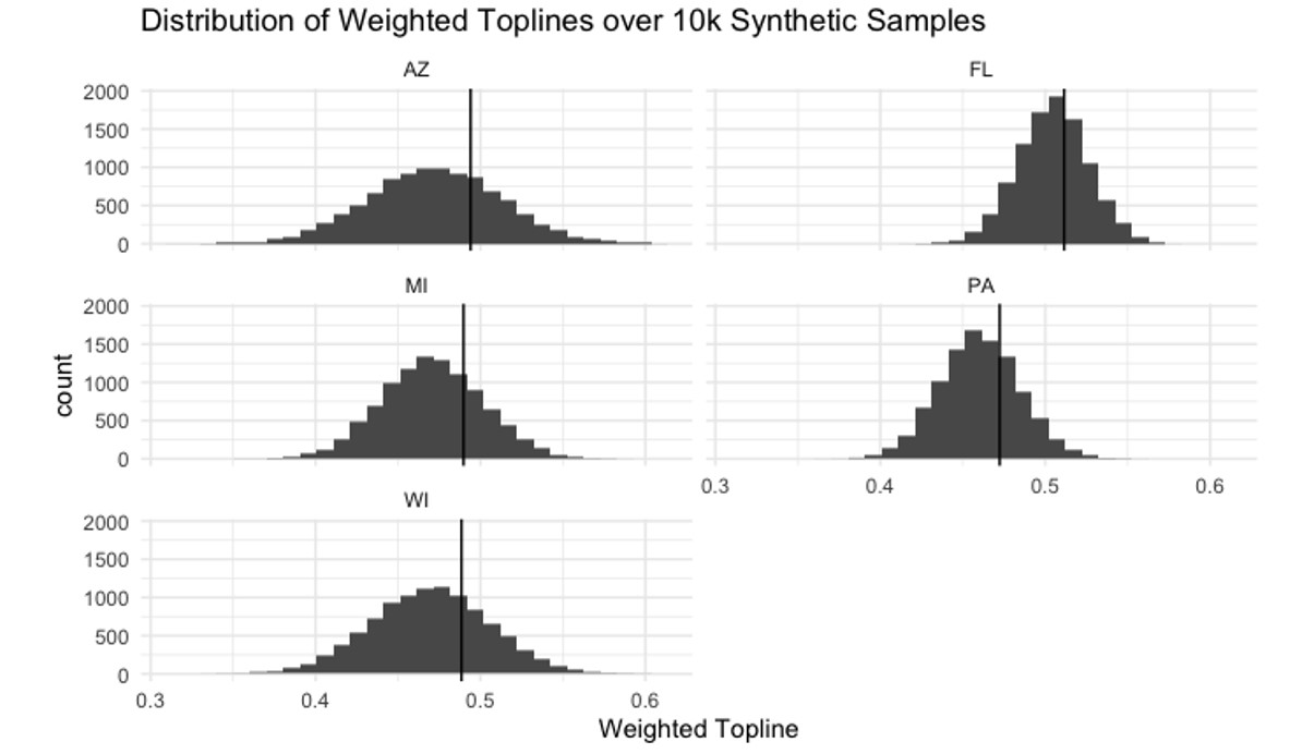
As the sample weights provided in the survey are themselves derived from comparing the joint distribution of demographic variables relative to the target population to correct for non-response bias, we could add them as one of the last variables to be synthesized after creating all the demographic variables. We can now calculate the weighted toplines for our 10K synthetic samples like pollsters often report, and compare them to the weighted toplines with the true data and sample weights as well as the final two-way Trump share in our five states.
| State | Raw Data Weighted Topline | Average of 10K Synthetic Samples Weighted Topline | Actual Two-Way Vote Share |
| Arizona | 49.3% | 47.2% | 49.8% |
| Florida | 51.1% | 50.4% | 51.7% |
| Michigan | 48.9% | 47.1% | 48.5% |
| Pennsylvania | 47.2% | 46% | 49.4% |
| Wisconsin | 48.8% | 46.9% | 49.6% |
Overall, we see that the raw weighted toplines and the average synthetic weighted toplines generally underestimate Trump’s actual performance, and that the synthetic toplines are systematically lower than the actual weighted toplines though, ultimately, the race would be correctly called.

Looking at the distribution of weighted toplines for our synthetic samples and adding a vertical line for the raw topline, we see that the synthetic datasets do in fact create toplines which are systematically lower than the raw data. The key challenges here relate to recreating the original sample weights and recognizing that the small errors underestimating Trump’s support which were present in the original survey propagated through the synthetic data generation, resulted in some synthetic samples which were completely off the final results. If some synthetic samples are better while others may be completely useless, how should we adapt our practices to account for the randomness that is inherent in the process of generating synthetic data?
Moving forward
While the best practices and paradigms under which research and inference should be conducted with synthetic samples are still the subject of fruitful debate among practitioners, we will all inevitably be working with synthetic data in the near future. Statistical agencies across the world like the US Census Bureau, the Office of National Statistics in the UK and EUROSTAT have been actively dedicating resources, time and funding on synthetic data.
We saw that while, on average, the inferences made from synthetic samples were relatively reliable, not all synthetic samples are created equally and the extent to which a single synthetic dataset could completely replace a raw dataset is still unknown. Repeatedly sampling and aggregating over many random draws may seem strange to non-statisticians, but it is actually one of the most widely used techniques in all domains of computational statistics with solid theoretical grounding.
Some researchers suggest a paradigm under which data collectors release multiple synthetic datasets to users for them to analyze, test and evaluate models on. The users would then send back their models, code or scripts which would then be run by the data collectors themselves on the original data and return the results back to the user.
Such efforts recognize that synthetic data can offer the key to striking the elusive balance between the rights of individuals and the good of the collective, capitalizing on those advancements in statistics and machine learning which open new and exciting avenues to help tackle some of the biggest challenges ahead.
References
https://www.census.gov/about/what/synthetic-data.html
https://www.synthpop.org.uk/get-started.html
https://edps.europa.eu/press-publications/publications/techsonar/synthetic-data_en
https://www.cs.cornell.edu/~shmat/shmat_oak08netflix.pdf
https://www.wired.com/2009/12/netflix-privacy-lawsuit/
Achilleas Ghinis is a Master’s student at KU Leuven studying statistics and data science, and a data scientist for BlueLabs. This article was a finalist for the 2022 Statistical Excellence Award for Early Career Writing. The 2023 writing award closes for submissions on 31 May 2023.


