This is an appendix to the May 2026 Significance magazine article Clear as a bell curve by D. S. Hill about a hidden structure in tonal music.
Method
- The 24 keys used in each collection covers the gamut of tonal music so there is no bias in this attribute. In addition, having the tonic located on all 12 possible notes ensures there is a breadth of keys, so there is no confound between key and register. That is, if all the pieces were in a narrow range of tonics close to middle C, then the peak of the aggregate could be higher than if the tonics were distributed more widely. But the complete set of keys spreads the distribution of the pitches right and left on the keyboard, which keeps register independent from key across the entire collection.
Analysis 1
- Enharmonic equivalents were counted as the same pitch class. Enharmonic equivalents are pitch classes (e.g., C# and D♭) that are on the same key of the piano
- The pitches were numbered from low to high and E(X) was calculated. The distribution was then mean-centred, with E(X) = 0. Higher pitches were numbered sequentially with positive integers and lower with negative.
- The actual distributions in Figures 1 through 5 are overlaid with either the quadratic line of best fit for Bach (R2 = .867) or for the others, G(0, σ), where σ is the sample standard deviation
- The relative brevity of Hummel’s preludes is a result of their purpose. In Hummel’s time, it was the practice for a pianist to play a brief prelude prior to the main piece. These could be improvised, previously composed by the performer or taken from a collection such as Hummel’s.
Analysis 2
- Random walks were generated with equal probability of remaining on the same pitch or moving ±1 semitone. A semitone is the interval between two adjacent keys on the piano – usually between white and black, but in the case of E to F and B to C, two white keys
- Starting points for each walk were drawn from an octave surrounding E(X). There were 50 runs on each of -6 and 6 and 100 on -5, . . , 5. The reason for half the runs on ± 6 is because that is the same pitch class (e.g., F# if C was 0). This doesn’t happen with the other positive/negative pairs. For example, if C was 0, -5 would be G and 5 would be F
- Each walk was approximately the same length as the average prelude for the corresponding composer:
- Bach: 682 notes
- Hummel: 129
- Chopin: 774
- Scriabin: 494
- Shostakovich: 714
- The walks were bounded by the range of each composer’s collection. Any time a walk reached a boundary, its position was reset to its original starting point. Hitting the boundary was rare, however, with the rate per 1000 steps ranging from 0.006 for Hummel to 1.04 for Bach
- The R2 and RMSE for each Random Walk Model were as follows:
| R2 | RMSE | |
| Bach | 0.735 | 0.006 |
| Hummel | -0.454 | 0.012 |
| Chopin | 0.863 | 0.004 |
| Scriabin | 0.889 | 0.004 |
| Shostakovich | 0.847 | 0.004 |
Analysis 3:
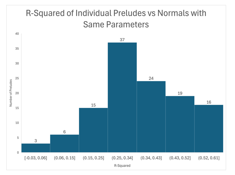
- The actual distribution of all 120 preludes was analyzed against their corresponding G(0, σ)
- The R2 for each was obtained using R (see histogram below)
- There was a meaningful fit for a strong majority of the preludes. 96 of the 120 preludes (80%) had an R2 ≥ .25. This is a satisfactory level of variance explained given that it uses only one explanatory variable (register)
- That is, many other compositional factors impact the choice of pitch: the key of the piece, motivic/melodic design, density of the harmonic texture, etc. The presence of these attributes limits the proportion of variance attributable to register alone
- A final factor is the relatively small number of pitches in each prelude compared to the total collection, with an average between 129.5 (Hummel) and 774.2 (Chopin).
- Generation of the linear combinations of bell curves:
- For each composer, 50 Gaussians had E(X) = -6 and E(X) = 6; 100 Gaussians had E(X) = -5,. . .,5. The standard deviations were drawn randomly from a range that placed the actual of each composer in the middle:
- Bach – 7 to 13
- Hummel – 8 to 16
- Chopin – 7 to 15
- Scriabin – 7 to 15
- Shostakovich – 9 to 17
- Values were drawn from a normal distribution; the cumulative normal distribution function (pnorm) was used to evaluate and truncate these values within the range of the corresponding composer before binning
- R2 and RMSE for Corresponding Random Walk and LCBC Models were as follows:
| Random Walk | LCBC | |||
| R2 | RMSE | R2 | RMSE | |
| Bach | 0.735 | 0.006 | 0.826 | 0.005 |
| Hummel | -0.454 | 0.012 | 0.921 | 0.003 |
| Chopin | 0.863 | 0.004 | 0.883 | 0.004 |
| Scriabin | 0.889 | 0.004 | 0.918 | 0.004 |
| Shostakovich | 0.847 | 0.004 | 0.856 | 0.004 |
Data, R code and supplementary methodological notes for the Significance article Clear as a bell curve:
https://github.com/DavidStuartHill/significance-clear-as-a-bell-curve


