Capture-recapture (CR) – or multiple systems estimation, as it is now also commonly known – is a method for estimating the size of an unknown population. It is an area of statistics that spans all levels of the career ladder from school syllabuses to Royal Statistical Society discussion meetings1, 2. It has an incredibly rich history, too, dating back to the 19th century when it was used to estimate fish populations3. More recently, in addition to its ecological uses, the method has been used to estimate human populations, such as victims of modern slavery4.
The ongoing appeal of CR must surely lie in the simplicity of the problem which it seeks to solve: estimating the size N of an unknown population, given multiple incomplete lists of subjects. By looking at the overlap between such lists, an estimate can be obtained for the number of subjects not appearing on any of the lists. This number is often referred to as the “dark figure”.
The above mention of school syllabuses might also bring to mind the work of William Shakespeare (1564–1616), arguably the most famous English writer of all time, whose corpus of work includes 38 plays and over 150 sonnets. As well as plays such as Macbeth, Hamlet and Romeo and Juliet, Shakespeare is well-known for his vocabulary, having introduced many new words and phrases into the English language (see Box 1). His vocabulary alone has been widely studied, with one aspect of particular interest being the size of his vocabulary, i.e. the number of words he knew.
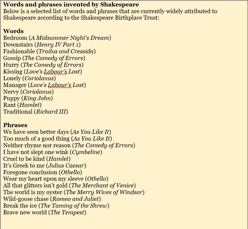
Box 1: Words and phrases invented by Shakespeare. Source: Shakespeare Birthplace Trust
An early estimate was made by the German-born philologist Friedrich Max Müller (1823–1900), who said, “[Shakespeare] produced all his plays with about 15,000 [different] words”. Yet Müller’s 19th century estimate was only relating to the number of used words, which, incidentally, is now believed to be around the 30,000 mark.
However, Shakespeare’s vocabulary can be said to comprise of not only the words he used in his plays, but also the more abstract set of words that he knew but never actually used. The first attempt to estimate the number of words in this latter category was made by Bradley Efron, of bootstrapping fame, and Ronald Thinet5. They looked at the counts for the number of words appearing once, twice and so on, and then used a Fisherian approach to estimate the number of words appearing zero times.
In this article, an alternative approach is considered: the standard CR method using log-linear models, as set out in 1972 by Fienberg6. By considering each of Shakespeare’s plays as a list of ni distinct words, an estimate can be obtained for the “dark figure” – i.e. the number of words Shakespeare knew but didn’t use in his plays – and hence N, the total size of his vocabulary.
The data
All of Shakespeare’s plays are free to download from the Folger Shakespeare Library. These can be used to construct a list of words appearing in each play, i.e. each play can be used to construct one list. Constructing a list for each play would yield 39 lists; however this would be excessive for CR, where the number of lists is usually between 3 and 6. Instead, 12 plays were randomly selected and grouped into three combinations of four (see Table 2) – essentially resulting in three separate data sets – which allows a comparison of estimates. These groupings were chosen randomly, but alternatively could have been grouped based on genres, e.g. comedies, tragedies and histories.
There is a certain level of ambiguity when creating these lists as to what constitutes a word and what constitutes Shakespeare’s vocabulary. For example, these lists were constructed using the Folger text versions and, unlike with dictionaries in the main, proper nouns – e.g. people’s names and places – were included. This is partly because, owing to the large number of words in each play, it would be a huge undertaking to sift through the words, removing proper nouns as appropriate. Similarly, the words in each list are case-sensitive, so some words have been counted twice.
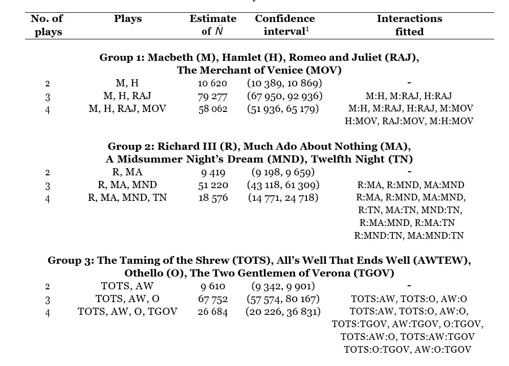
Table 2: A summary of the models fitted. 1 This is a 95% confidence interval based on the profile likelihood.
A summary of CR
To give a brief summary of the CR (multiple systems estimation) model, suppose there are two just plays, say, Macbeth (M) and Hamlet (H), hence two lists. Every word in Shakespeare’s vocabulary can be allocated to one of four mutually exclusive categories. It is either: included in both M and H, included in M but not in H, included in H but not in M, or included in neither M nor H (see Table 1 in Box 2). While the number of words falling into the first three categories can be counted, the number falling into the latter category cannot be counted and requires estimation. To estimate this number, the following three key assumptions are made7 :
- Each play is drawing from the same vocabulary (“closed population”).
- Each word has the same probability of appearing in a given play (“homogeneous capture probabilities”).
- Each play is independent (“independence of lists”).
Assumption 1 seems reasonable enough, although Shakespeare’s vocabulary and literary style, like that of other authors, may have changed over time. Plus, rather interestingly, there has been an argument, too, as to whether Shakespeare did indeed write all of his plays. Assumption 3 also seems reasonable; although Shakespeare may have been influenced by other playwrights. The sticking point comes with assumption 2: clearly words such as “and” and “the” are far more likely to appear than other words. Plus, for example, Macbeth, a tragedy set in Scotland, requires different types of words (e.g. different place names) to, say, Much Ado About Nothing, a comedy set on Sicily.
The good news however is that, when there are more than two lists, we can partly relax this assumption by including interactions in the model. Yet this can be a contentious issue8 as model selection can greatly impact the subsequent estimates.
When there are four lists, there are 15 (rather than 3) observed counts. These counts are given in the Venn diagrams in Figure 1.
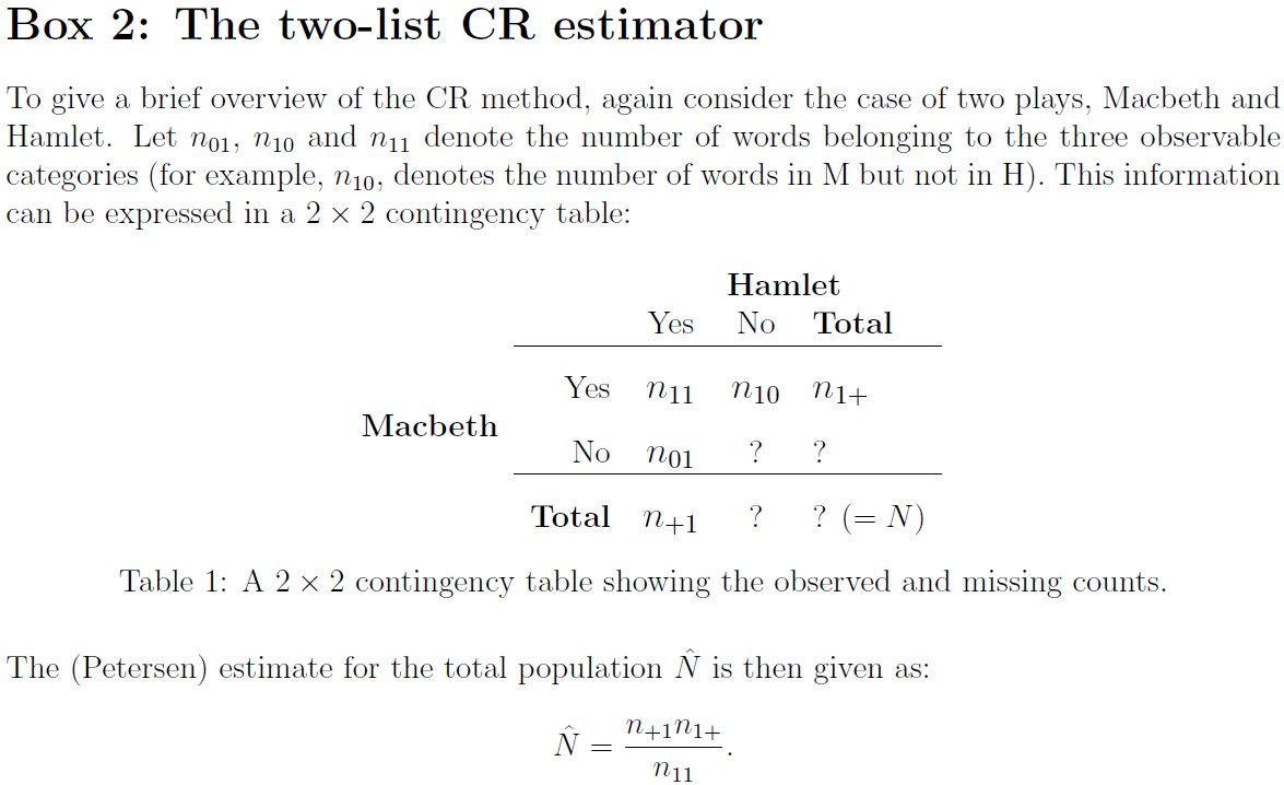
Box 2: The two-list CR estimator
The results
For each of the three groups, the effect of adding a list is assessed. For example, for Group 1, consisting of Macbeth, Hamlet, Romeo and Juliet (RAJ) and The Merchant of Venice (TMOV), an estimate is first obtained – 10,618 – using M and H, only. Then secondly an estimate is obtained – 79,231 – for when RAJ is added. Then thirdly an estimate is obtained – 58,044 – for when TMOV is also added. A similar approach was taken for Groups 2 and 3. For the models involving three or four lists (plays), a backward elimination routine (using AIC) was used to select the final model.
The estimates are presented in Table 1 in Box 2. The results from the three groups are remarkably similar in the pattern they take. When there are just two lists, for example, the estimates for the size of Shakespeare’s vocabulary is around 10,000. Based on other studies, this is clearly an underestimate – far more used words have been identified – and thus demonstrates the practical limitations of two-list CR.
The 3- and 4-list cases are more insightful. The 3-list cases consistently produce higher estimates than the 4-list cases; the 3-list estimates are in the range 51,000-79,000 whereas the 4- list estimates are in the range 18,000-58,000. Therefore, perhaps 25,000 and 79,000 can be taken as very rough lower and upper bounds, respectively, for the number of words in Shakespeare’s vocabulary.
Conclusion
In some ways, this article illustrates the limitations of CR. While it is undoubtedly an elegant approach – and can provide a valuable insight into the size of an unknown population – it is also difficult to obtain reliable, consistent estimates. The model is particularly sensitive to slight changes in the model fitted, e.g. including or omitting an interaction can greatly impact the final estimate.
Yet, regardless of what the true value is for the size of Shakespeare’s vocabulary, the results indicate that Shakespeare only used a fraction of the total words he actually knew, meaning the loss of words that, alas, will never grace the English language.
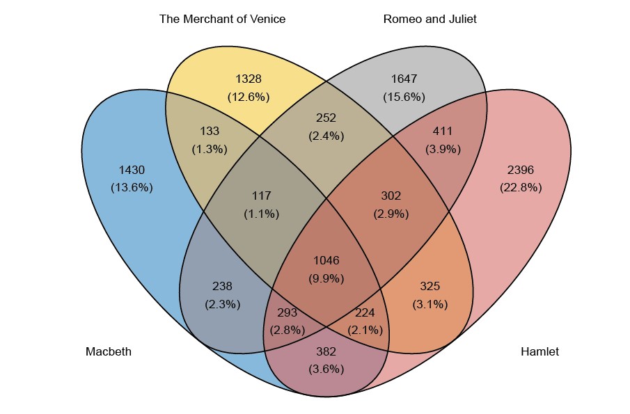
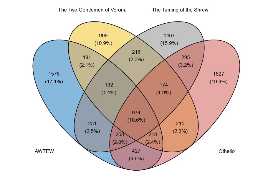
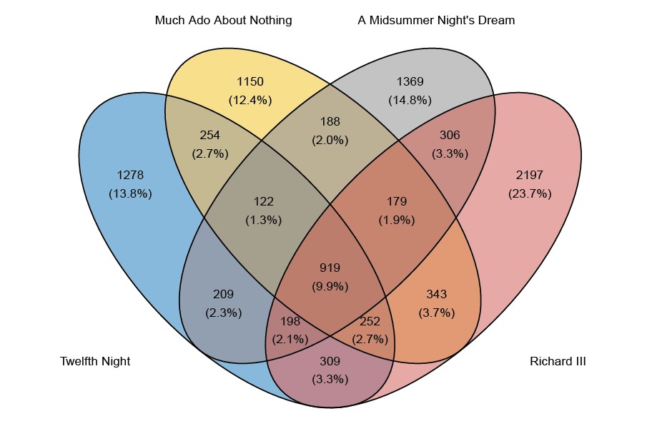
Figure 1: Venn diagrams giving the counts for the number of words falling into each category. For example, in the top plot, the 1430 in the blue portion on the left-hand side relates to the number of words that appear in Macbeth but do not appear in The Merchant of Venice, Romeo and Juliet and Hamlet. (AWTEW = All’s Well That Ends Well). In CR, the number to be estimated is the number that lies in the white space outside the Venn diagram, that is, the number of words that do not appear in any of the plays.
Acknowledgments Many thanks to Kelly Zou, member of the Significance editorial board, for the helpful comments she made on the article.
References
1. Silverman, B. W. (2020) Multiple-systems analysis for the quantification of modern slavery: classical and Bayesian approaches (with discussion). Journal of the Royal Statistical Society Series A: Statistics in Society, 183, 691–736.
2. Dunne, J. and Zhang, L.-C. (2023) A system of population estimates compiled from administrative data only (discussion forthcoming). Journal of the Royal Statistical Society Series A: Statistics in Society. URL: https://doi.org/10.1093/jrsssa/qnad065. Qnad065.
3. Goudie, I. B. and Goudie, M. (2007) Who captures the marks for the Petersen estimator? Journal of the Royal Statistical Society: Series A (Statistics in Society), 170, 825–839.
4. Petersen, C. G. J. (1896) The yearly immigration of young plaice into the Limfjord from the German Sea. Report of the Danish Biological Station, 1895, 1–48.
5. Efron, B. and Thisted, R. (1976) Estimating the number of unseen species: How many words did Shakespeare know? Biometrika, 63, 435–447.
6. Fienberg, S. E. (1972) The multiple recapture census for closed populations and incomplete 2k contingency tables. Biometrika, 59, 591–603.
7. Manrique-Vallier, D., Price, M. E. and Gohdes, A. (2013) Multiple systems estimation techniques for estimating casualties in armed conflicts. In Counting Civilian Casualties: An Introduction to Recording and Estimating Nonmilitary Deaths in Conflict (eds. T. Seybolt,
8. Whitehead, J., Jackson, J., Balch, A. and Francis, B. (2019) On the Unreliability of Multiple Systems Estimation for Estimating the Number of Potential Victims of Modern Slavery in the UK. Journal of Human Trafficking, 1–13.
James Jackson is a research associate at the Alan Turing Institute. This article was shortlisted for the 2023 Statistical Excellence Award for Early Career Writing.
*Hamlet to Polonius, Hamlet, Act II, scene II


